An interactive app for spatially explicit capture–recapture

Introduction
Main screen
Habitat mask
Summary
Options
References

Introduction

This Shiny application is an interactive interface to parts of the R package secr (Efford 2022). The current source code is available from https://GitHub.com/MurrayEfford/secrapp. The step-by-step guide overlaps in scope with this document and may ultimately replace it.

Documentation of secr is available at www.otago.ac.nz/density. For example:

secr-manual.pdf (details of each function)
secr-datainput.pdf
secr-overview.pdf

The analyses available through the Shiny app are a subset of those in secr. Support for multi-session analyses is limited.

TIP: on small displays, running your browser in full-screen mode will avoid the need to scroll down (often F11 will get you there; otherwise try the options menu of the browser).

Main screen

Use settings on this page to input data and fit simple models.

Data input

By default, input is from two text files, one for the detector layout and one for detections ('captures') of known individuals. Excel files may also be used. Alternatively, secrapp may read the complete secr capthist object from a .rds file, or use one of the builtin datasets.

Detector layout

The detector layout file typically should have three columns (trapID, x, y) with no headers. These may optionally be followed by binary usage codes (0/1), one per occasion. Columns after a '/' are interpreted as detector covariates. Headers are required for input from Excel files.

Options for detector type follow secr (Efford (2022)): “multi” refers to a multi-catch trap; “proximity” to binary proximity detectors, and “count” to detectors that yield integer counts. Counts are assumed to be Poisson-distributed. Data from searches of areas or transects use the types “polygon”, “polygonX”, “transect” or “transectX” (Efford 2011; see also secr-polygondetectors.pdf).

If detector covariates are included then one or more covariate names should be provided (without quotes, separated by commas).

Optional arguments separated by commas may be used to customise input (e.g., skip, which is passed through read.traps to read.table).

Captures

Two formats are allowed, as in DENSITY or secr; 'trapID' uses four columns (Session, AnimalID, Occasion, TrapID) and 'XY' uses five (Session, AnimalID, Occasion, X, Y). Supplementary columns are interpreted as individual covariates.

If individual covariates are included then the correct number of covariate names should be provided (without quotes, separated by commas).

Optional arguments separated by commas may be used to customise input (e.g., skip, which is passed to read.table).

A filter may be applied to captures loaded from text files or spreadsheets. Clicking on the 'filter' link in the Captures panel opens an additional text input. Text entered in this box should be one or more valid argument(s) for the secr function subset.capthist. Filtering is switched off when 'filter' is clicked again and the text input disappears. It is best to enter the filter criterion before browsing to the captures file or spreadsheet.

Table. Filtering criteria (main arguments of subset.capthist)

Argument	Selects	Example	Note
subset	individuals	`covariates(ch) == "M"`	assuming one individual covariate with values “F”,“M”; == not =.
occasions	sampling occasions	`occasions = 1:3`	limit to first 3 occasions
traps	detectors	`traps = traps(ch)$x < 500`	only western part of array
sessions	sessions	`sessions = 1`	may select one or more sessions

Each argument is a vector of subscripts that may be logical- (length equal to the relevant dimension of ch), character- or integer-valued, except that occasions should be specified by their number. Arguments occasions, traps and sessions should be named, but may be shortened (e.g. occ = 1:3). Criteria may be combined (separated by commas).

Selecting individuals (argument subset) can be problematic, especially from multi-session data. If covariates(ch) has more than one column then specify with, e.g., covariates(ch)$sex == "M".

To select individuals from multi-session data on the basis of a covariate it is best to specify the subset as a function. This is illustrated in the Examples for subset.capthist. Given a dataset with individual covariate 'Sex' (named in the 'Covariate names' input) we might select males with function(x,sex) covariates(x)$Sex==sex, sex = "M". If filtering fails then check the covariate names, including capitalisation.

The Summary table includes the filter text unless that summary field is deselected.

Model

Detection function	HN	halfnormal	$ \small g(d) = -g_0 \exp\{-d^2/(2\sigma^2)\} $
	HR	hazard rate	$ \small g(d) = -g_0 (1 - \exp(-(d/\sigma)^{-z})) $
	EX	negative exponential	$ \small g(d) = -g_0 \exp(-d/\sigma) $
	HHN	hazard halfnormal	$ \small \lambda(d) = -\lambda_0 \exp(-d^2/(2\sigma^2)) $
	HHR	hazard hazard rate	$ \small \lambda(d) = -\lambda_0 (1 - \exp(-(d/\sigma)^{-z})) $
	HEX	hazard negative exponential	$ \small \lambda(d) = -\lambda_0 \exp(-d/\sigma) $

Likelihood	maximize full likelihood or likelihood conditional on $ \small n$
Distribution	distribution of number detected $ \small n$
Mixture hcov	name of individual covariate

The supported detection functions are a subset of those allowed in secr (currently 'HN', 'HR', 'EX', 'HHN', 'HHR', 'HEX'). These relate either the probability (g(d)) or hazard ($ \small \lambda$) of detection at a particular detector on a particular sampling occasion to the distance $ \small d$ of the detector from its home-range centre. The probability of detection is $ \small g(d) = 1 - \exp \{ - \lambda(d)\}$.

The Distribution radio button toggles between two models for the number of detected individuals $n$. The “Binomial” option corresponds to fixed number $N$ in the masked area and a binomial point process for the distribution of activity centres. The “Poisson” option corresponds to Poisson $N$ and a Poisson point process for activity centres.

The Mixture hcov select input allows the user to choose a variable defining a 2-level mixture class from among the individual covariates. This is passed to secr.fit as the argument 'hcov'. The covariate should take two non-missing values (e.g., 'F','M'); missing values are allowed. The mixing proportion 'pmix' is included in the model automatically when hcov is specified. To estimate mixture-specific values of a parameter include ~h2 in its formula (e.g., lambda0~h2). See secr-finitemixtures.pdf for more.

Other arguments separated by commas may be used to customise the call to secr.fit. Attempts here to change 'capthist', 'mask', 'model' or 'detectfn' are ignored, and 'trace' is always FALSE.

Model formulae may be edited using pre-defined predictors or covariate names as described in secr-overview.pdf. Time covariates ('timecov') and session covariates ('sessioncov') may be specified in Other arguments. There is no provision for time-varying detector covariates.

The Habitat mask box reports attributes of the mask currently defined on the Habitat mask screen; use the edit link to vary these.

Time limits

The application is designed for small- to medium-sized models. An internal algorithm predicts the execution time by evaluating the likelihood once and making a simple extrapolation. The prediction is quite rough. When the predicted time exceeds a lower threshold ('timewarning', default 0.5 minutes) a dialog box asks the user for confirmation before proceeding. If the predicted time exceeds an upper threshold ('timelimit', default 10 minutes) then execution aborts, with a notification at the lower right of the screen. The thresholds may be changed in the R code of the app.R file (near the top).

Actions

Fit model	Fit closed-population SECR model
Reset all	Reset all input options to defaults
Bookmark	(see Bookmarking)

'Reset all' does not delete Summary results from the current session. Use the buttons on the Summary page to manage the summaries. Summary results will be lost if you close the application without downloading to a local file.

The option 'Switch to secrdesign' appears once a model has been fitted if the detection function is HHN or HEX and the detector type is multi, proximity or count. This opens 'secrdesignapp' on the Otago University server in a new browser window. Settings and parameter estimates are transferred automatically. Detector locations are not transferred; they should be provided either by selecting the file in secrdesignapp, or by the usual options (Grid, Line, Region).

Results

Values in the Results window are updated automatically when the inputs change.

The default 'results' vary depending on the inputs

summary of detector layout only
summary of capthist object (detector layout + detections)
summary of fitted model
user-specified code, possibly referencing the capthist (ch) or fitted model (fitted), or displaying a help topic from 'secr' (e.g., ?detectfn).

Once a model has been fitted it is possible to select

summary of fitted model
table(s) of estimates from predict
table of derived (Horvitz-Thompson) estimates

The 'hide' button temporarily suppresses the summary output.

Tabbed code and plots

Plots update automatically. Any plot may be saved by right-clicking on the image.

Code

R statements for the main operations. These expand once you browse to specific detector and capture files.

The statements may be copied and pasted into an R session. It is assumed that input files are in the current folder; you may need to change this with setwd().

Array

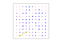
A plot of the current detector layout. Detections are overplotted if they have been uploaded.

By default, the locations of one animal are highlighted and its ID, number of detections and observed range length (ORL) appear in a box. Suppress this by selecting animal '0'. Click on the plot to select an individual.

A session selector is shown for multi-session data. Changing the session changes the plot displayed on this tab, and on some others (Buffer, Pxy, Dxy); it does not affect model fitting.

Once a model has been fitted, ticking 'fxi contour' displays a contour plot of probability density contours for the activity centre of the current animal. This may fail if the mask spacing is too small.

Moves

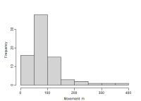
Histogram of distances between the successive detections of each animal. The bar width is determined internally from an integer value provided to the 'breaks' argument of hist. You can vary the 'Nominal breaks' setting (small changes have no effect because of the algorithm used by hist).

Summary statistics appear in a box to the right. “Approx HN sigma” is computed with the secr function RPSV(capthist, CC = TRUE); the approximation is an underestimate, especially when the detector array is small.

Non-exclusive detector types (proximity, count etc.) allow multiple detections on a single occasion, and the order of these detections is unknown. The distances then depend on the arbitrary within-occasion ordering of detections.

For multi-session data the displayed histogram is for the current session (see Array tab), unless 'Combine sessions' has been selected on the Options screen. When sessions are combined, the default is to include session-session movements. This may be changed on the Options screen.

Detectfn

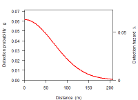
Fitted detection function on the hazard and probability scales.

Buffer

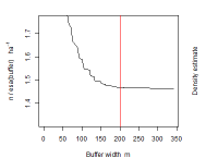
Predicted effect of buffer width on density estimates. The plot is generated with esa.plot(fit). A red vertical line indicates the buffer that was used (there is no line when the mask has been read from a file).

Pxy

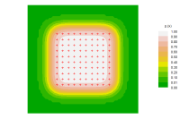
Contours of the overall detection probability $ \small p_\cdot(\mathbf x)$ under the fitted model ('Pxy' is the label that has been used for this quantity in the Windows application Density). Settings in Options toggle the display between filled and unfilled contour plots, and determine whether contours are labelled. The requested contour levels are 0.1, 0.2, …, 0.9, but higher contours may be missing. Click on the plot to find the value at a point.

Dxy

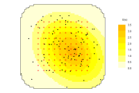
A plot of the fitted density model with various optional overlays:

detector locations (red crosses)
petal plot of detections
one simulated population from the fitted model
circles with 95% home range for each centre in the simulated population

Power

Two styles of plot are offered (see Options | Power plot)

Power for test of null hypothesis

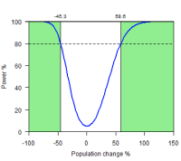
Probability of detecting a change in density in a 2-survey comparison as a function of effect size for a given expected $ \small \mbox{RSE}(\hat D)$. See Efford and Boulanger (2019) for the computation method.

Effect size is the ratio of final density $ \small D_2$ to initial density $ \small D_1$ expressed as a percentage. The alpha level is specified in Options (default $ \small \alpha = 0.05$).

The curve is initially computed for the rule-of-thumb RSE from the current design. Use the slider to vary this. Especially, consider adding a safety margin for underestimation of RSE.

The default method assumes that $ \small \mbox{RSE}(\hat D)$ is the same in the initial and final surveys. It is more likely that $ \small \mbox{RSE}(\hat D)$ will increase as density declines. An adjustment is applied to the final RSE when the 'Adjust RSE' box is ticked: $ \small \mbox{RSE}(\hat D_2) = \sqrt {D_1/D_2} \mbox{RSE}(\hat D_1) $.

Confidence interval for population change

As an alternative to conventional power analysis we can construct intervals for the estimated ratio of densities, given the true ratio and the sampling errors. The interval is the region between the upper and lower curves for a given true population change on the x axis.

Habitat mask

Either construct a habitat mask from scratch ('Build') or read mask coordinates from a text file ('File').

The 'Suggest width' button runs the secr function suggest.buffer which is currently available only for point detectors (not polygon types). The algorithm requires that captures have been loaded.

A mask built by buffering around a detector array may include known non-habitat. Polygon data from an ESRI shapefile may be used to include or exclude sites from the mask.

Mask covariates are used to build spatial models of density (D). Covariate data may be added from a spatial data source - either a polygon shapefile, a SpatialPolygonsDataFrame stored in an .rds file, or a text file in the format used for habitat masks (below). Covariate values at each mask point are inferred from spatial overlap (shapefile or SpatialPolygonsDataFrame) or the nearest source point (mask file).

A mask text file should have a header line. The first two columns ('x', 'y') are read as the x- and y-coordinates. Further columns are assumed to represent covariates and their names may be used in formulae for density.

Summary

The table on this page has one column for each model fit or other summary; summaries are added automatically when models are fitted.

The displayed table includes only selected analyses. Users should ensure AIC comparisons are valid across the selected analyses (use same data and compatible model structure).

The table may be downloaded as a comma-separated text file or in the RDS format (use readRDS to restore in R). The table is transposed on download so that scenarios become rows.

Options

These should be self-explanatory. Experiment if in doubt.

Model fitting

Maximization method

The default (Newton-Raphson in function nlm) is generally OK. Nelder-Mead in function optim is slower and somewhat more robust with difficult likelihood surfaces.

Number of cores

Multithreading allows some operations to be performed in parallel for faster model fitting. The number of cores (ncores argument of secr::secr.fit) may be set manually. The maximum allowed by secrapp is the smaller of 24 and the number of cores available (including virtual cores)[1]. The default number of cores is half the maximum.

[1] The limit of 24 is arbitrary. It stops a user from hogging a vast number of cores in some environments.

Time limit

A model will not be fitted if the predicted time exceeds a limit, currently 10 minutes. The prediction is quite rough as there is no obvious way to anticipate the number of likelihood evaluations that will be required.

Bookmarking

NOTE: Bookmarking is disabled in secrapp 1.4 owing to a problem in Shiny.

References

Borchers, D. L. and Efford, M. G. (2008) Spatially explicit maximum likelihood methods for capture–recapture studies. Biometrics 64, 377–385.

Efford, M. G. (2011) Estimation of population density by spatially explicit capture–recapture analysis of data from area searches. Ecology 92, 2202–2207.

Efford, M. G. (2022) secrdesign: Sampling design for spatially explicit capture–recapture. R package version 2.6.0. https://CRAN.R-project.org/package=secrdesign

Efford, M. G. (2022) secr: Spatially explicit capture–recapture models. R package version 4.5.2. https://CRAN.R-project.org/package=secr

Efford, M. G. and Boulanger, J. (2019) Fast evaluation of study designs for spatially explicit capture–recapture. Methods in Ecology and Evolution 10, 1529–1535.

Detection function	HN	halfnormal	\( \small g(d) = -g_0 \exp\{-d^2/(2\sigma^2)\} \)
	HR	hazard rate	\( \small g(d) = -g_0 (1 - \exp(-(d/\sigma)^{-z})) \)
	EX	negative exponential	\( \small g(d) = -g_0 \exp(-d/\sigma) \)
	HHN	hazard halfnormal	\( \small \lambda(d) = -\lambda_0 \exp(-d^2/(2\sigma^2)) \)
	HHR	hazard hazard rate	\( \small \lambda(d) = -\lambda_0 (1 - \exp(-(d/\sigma)^{-z})) \)
	HEX	hazard negative exponential	\( \small \lambda(d) = -\lambda_0 \exp(-d/\sigma) \)

What is secrapp?

What does secrapp do?

Where can I get help?

References

Data input

Model

Actions

Results

Summary

Fields

Analyses

Download

Data Import/Export

Model fitting

Summary

Array plot

Pxy contour plot

Dxy plot

Moves histogram

Power plot

Hypothesis test

An interactive app for spatially explicit capture–recapture

Contents

Introduction

Main screen

Data input

Detector layout

Captures

Model

Time limits

Actions

Results

Tabbed code and plots

Code

Array

Moves

Detectfn

Buffer

Pxy

Dxy

Power

Power for test of null hypothesis

Confidence interval for population change

Habitat mask

Summary

Options

Model fitting

Maximization method

Number of cores

Time limit

Bookmarking

References

secr app 1.4

This Shiny application provides an interface to the R package 'secr', version 4.5.3 .

Copyright 2019, 2022 Murray Efford

For further information see

Citation

Analyses with this interface should refer to the parent package, secr. The citation for the current version is -

Efford, M. G. (2022). secr: Spatially explicit capture-recapture models. R package version 4.5.3.

https://CRAN.R-project.org/package=secr.