2 Getting started with R

R Environment

The first step is to install R and RStudio, you can do so by following these links.

Install R. Choose the appropriate download for your operating system.

Install RStudio. Select the free version of RStudio, this has everything you need.

Once these are both successfully installed, open RStudio. This is what it should look like:

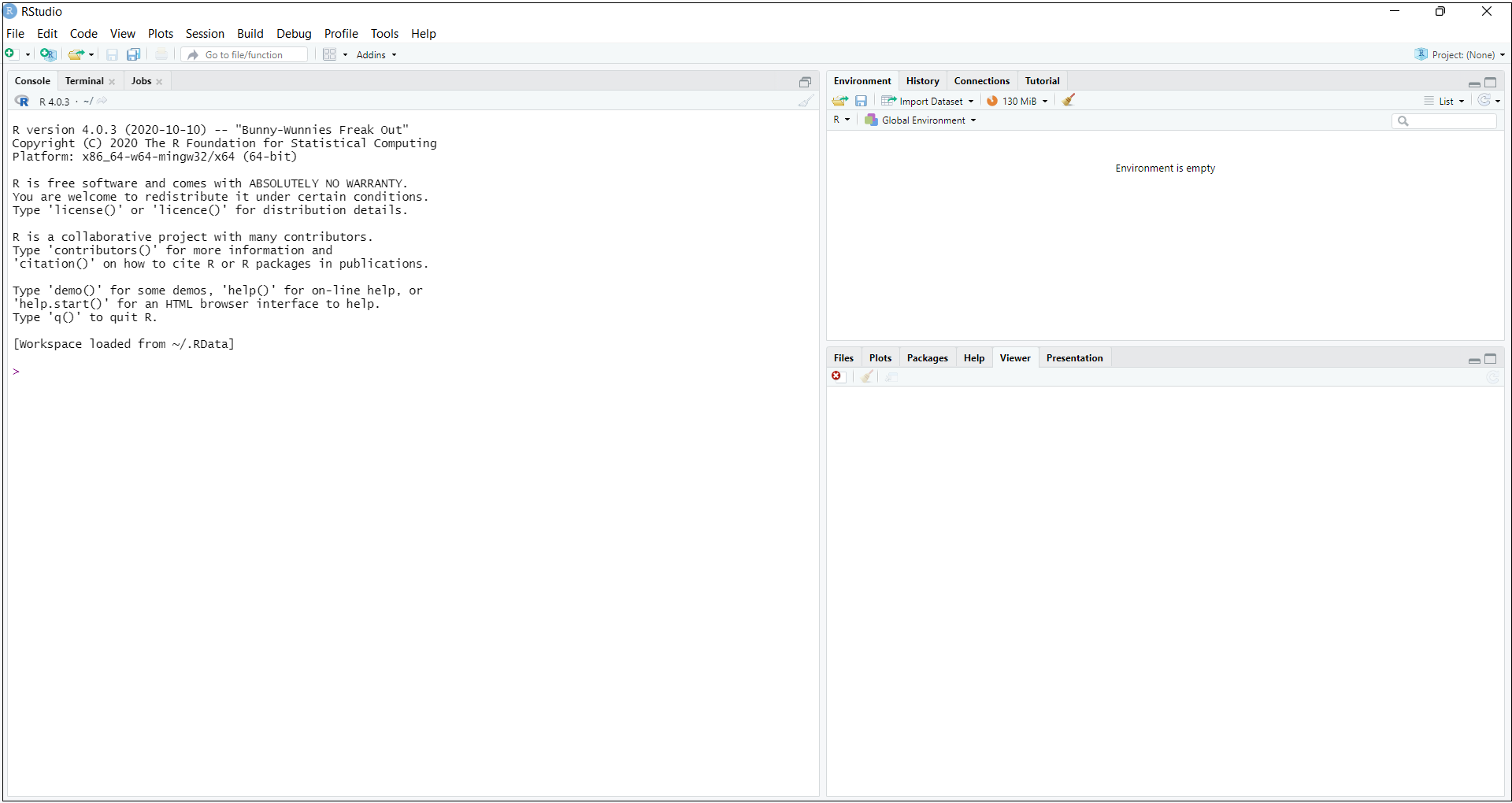
The left window is your Console. You can type and execute code directly here at the >, but this is not recommended as it does not allow you to save or make edits to your code.

A more efficient approach is to type code into a Script before running it in the console, giving you the option to save your work. An R script is essentially a blank document where you type code, then execute it by clicking the relevant line followed by “Run” in the top right of the script window.

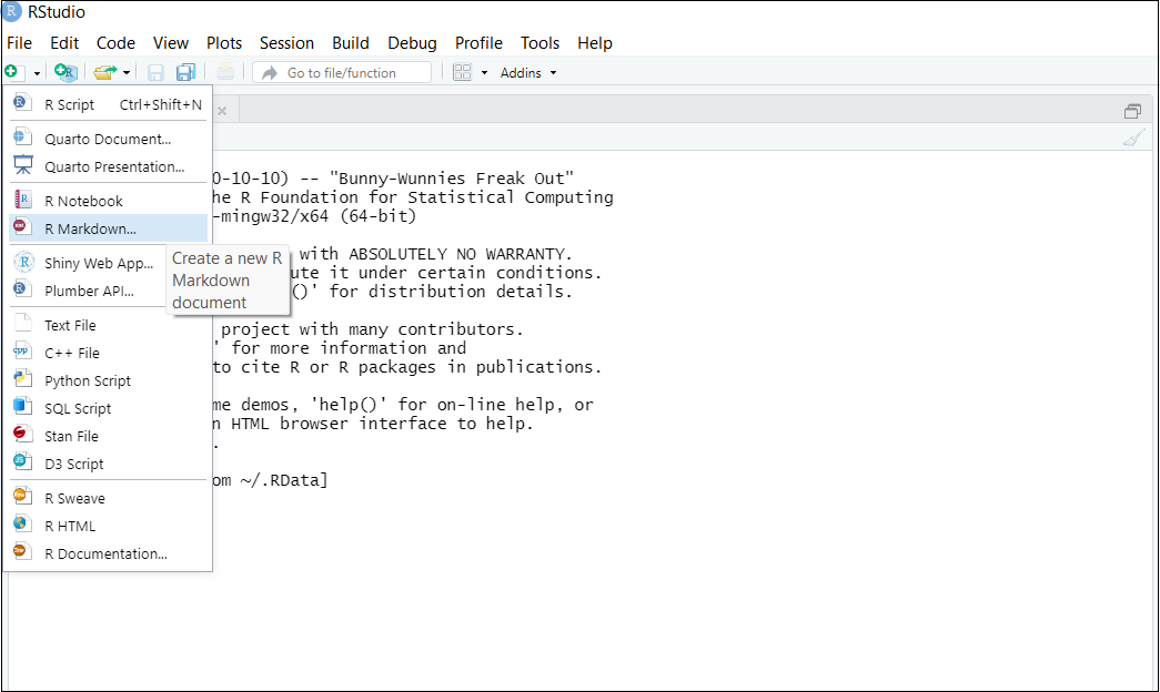
For these lessons, we suggest using an R Markdown script. This format combines code, output (calculations, plots, etc.) and text into a single document. You can open one in the top left window as shown below. First click the “New File” button with the green plus sign (just below “File”), followed by “R Markdown …” .

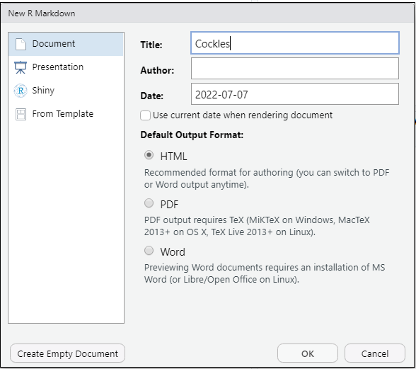
Give your script an appropriate title, then click OK to open in.

Here is what an R Markdown script looks like:

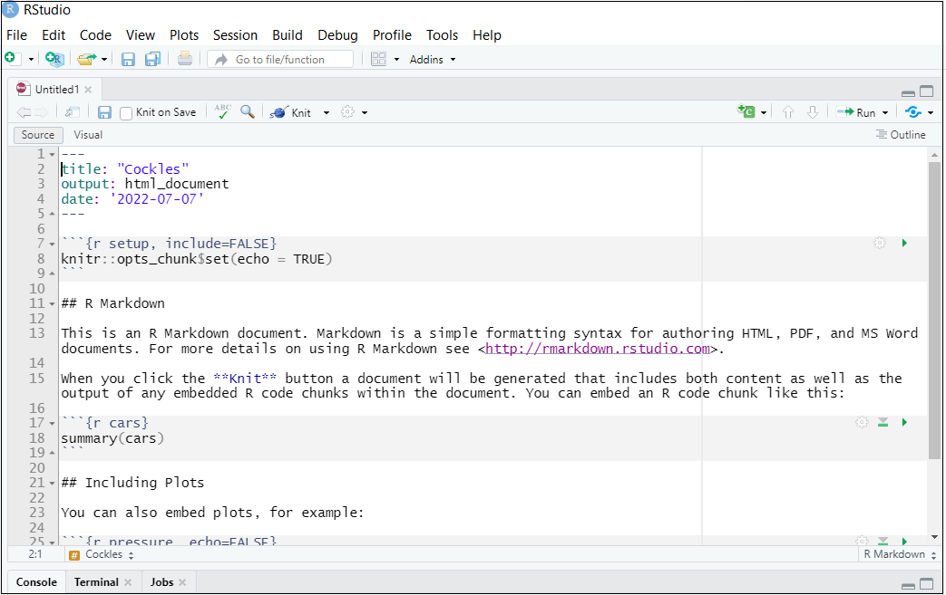
The grey areas are called “chunks” and contain code. To execute a chunk, click the small green arrow on the far right. Results will be printed below the code in your document. The downwards pointing white arrow just to the left of this executes all previous code chunks.

You can practice this with the example code that is initially provided when you open a Markdown script. You can then delete this code as it is not needed for the functioning of your Markdown or any of the subsequent lessons.

The Environment tab in the top right window indicates the objects that you have in your R environment (such as vectors and data frames). This will make more sense once you begin running code and see objects appear here.

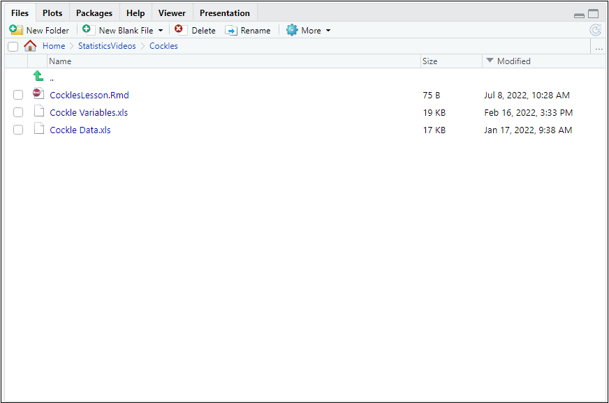
The Files tab in the bottom right window shows your working directory, which is the folder R can load data from during your session.

For each lesson you should first save the relevant data as well as your R Markdown script into a folder. Then use ctrl+shift+h within RStudio and navigate to this folder to set your working directory.

Executing code

The cornerstone of an R Markdown file is the executable code chunk. You have seen above how to run an existing chunk. There are 3 options for creating a new chunk.

Use the “Insert a new code chunk” button in the top right of your script window, and select R.

Manually type in the chunk. ```{r} followed by ``` a few lines below.
Copy and paste an existing chunk, and edit the code contents.

To input code, type directly into a chunk or the console. Note that R is case and punctuation sensitive so make sure to check this if you’re getting an error (particularly $\verb!object not found!$). Aside from within object (variable, data frame) names, R is not space sensitive. Don’t worry about spaces in your code, aside from ensuring readability.

You can include comments within code chunks using # followed by your comment. This can be useful to provide information about your code and to remind yourself what it is doing. The # in front prevents this text from executing when the chunk is run.

If you wish to save your Markdown file to come back to, simply click the “Save current document” (floppy disk symbol) in the top left of your script. A clue that the most recent copy of your file has not been saved is the file name showing up in red, this changes to black after all changes are saved.

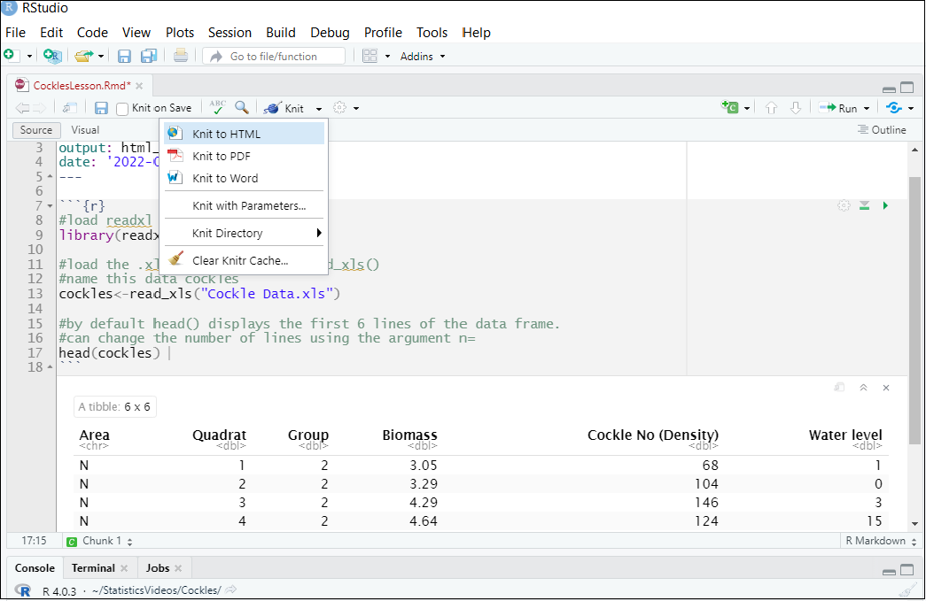
Once you are happy with your Markdown document (and all chunks run without errors), you can knit this to create an independent output file (click the “Knit” button in the top left of your script). This will contain all the results of your analysis in an attractive format, and can be viewed without needing to run RStudio. The default knitted file type is .html, as this can be compiled and viewed without any additional software. It is also possible to knit to word and .pdf. Knitting to .pdf is more involved and requires installation of software such as MiKTeX, instructions are available on the Internet if you would like to do this.

Now you have learnt the basic concepts of utilising R and Markdown environments, it’s time to take a look at we can do using these tools.

Important Information

The following explanations will be most beneficial if you work through them explicitly.

Use the previous instructions to open an R markdown script within RStudio.

As you read through the subsequent sections, copy the code provided into chunks within your script and run it to see the results.

Storing and Accessing data

To store any value in R you must assign it a name. This saves the value in the global environment, and allows us to retrieve the value by typing the name.

You can assign names using the commands <- or =

Code

#ASSIGN the value 5 to the name n
n<-5  

#ASSIGN the logical value TRUE to the name honest
honest="TRUE"

Code

#calling the object names RETRIEVES the values 5 and TRUE
n

[1] 5

Code

honest

[1] "TRUE"

Code

#using two subsequent equals signs (==) CHECKS if objects are equal
n==5

[1] TRUE

Code

honest=="FALSE"

[1] FALSE

There are two key formats that allow you to combine multiple data points, allowing you to more effectively store data in R.

The first is a vector, this is a string of values.

The values can be numeric (numbers), character (strings of letters), logical (TRUE or FALSE, also represented by T or F) or a combination of all three.

Numeric and character vectors are sometimes factors, also known as categorical variables. This is the case when the numbers or words that make up the vector entries are actually codes for particular categories (levels). For example, a vector of values of the factor variable hair colour may have the levels “dark” (coded for black or brown hair), “light” (coded for auburn or blonde hair), and “other” (coded for other hair colours).

A vector is created using the function c(), with the entries separated by commas. You can extract entries from a vector by subsetting with square brackets [ ] and specifying the position of the value you would like.

These processes are shown below:

Important Information

Make sure to run this code chunk now, as these objects will be used in later code demonstrations.

Code

#create a numeric vector with five numbers and name it x
x<-c(3,4.5,20,1.6,15)  

#create a vector by combining two sequences of numbers(1 to 50 and 25 to 55), name it w
w<-c(1:50,25:55) 

#create a vector with a logical value and two character values, name it z
z<-c(TRUE,"pidgeon","dove") 

#create a vector with character values representing levels of the factor variable hair colour
hair.colour<-c("other","light","light","dark","other","dark","dark") 

#extract the third entry of z
z[3]

[1] "dove"

The second way of storing data is in a data frame. This is a two-dimensional object, made up of rows and columns. You can imagine a data frame as a collection of vectors, i.e. each column is a vector and the rows make up its entries.

Like vectors, the values of a data frame can be numeric (numbers), character (strings of letters), logical (TRUE or FALSE) or a combination of all three. Character values are almost always representative of factor variables in data frames however. Data frames typically have a heading at the top of each column indicating the variables they contain observations from.

Data frames can be created from scratch using the data.frame() function. The columns of this data frame y are called “Name”,“Bird”, “Size”, and “Seen”. These are each made up of vectors of values:

Important Information

Make sure to run this code chunk now, as these objects will be used in later code demonstrations

Code

#create a data frame with 3 columns (each containing 5 rows) and name it y
y<-data.frame(Number=c(1:5),Bird=c("Tui","Fantail","WaxEye","Kingfisher","Bellbird"),
              Size=c("Large","Small","Small","Medium","Medium"),Seen=c(4,7,3,1,5)) 

#view the contents of y
y

  Number       Bird   Size Seen
1      1        Tui  Large    4
2      2    Fantail  Small    7
3      3     WaxEye  Small    3
4      4 Kingfisher Medium    1
5      5   Bellbird Medium    5

It is also possible to load an existing data frame into R, in fact, this is typically the first step of data analysis.

The functions to do this follow the general form read....() e.g read.table(), read.csv() etc. depending on format the data frame is saved in. Within the brackets, you specify the file name in quote marks “…”, along with other information depending on the function.

The lessons on this site use Microsoft Excel spreadsheet data, which is read into R using read_xls(). The data frames created by this function are actually tibbles, you can read more about these on the internet but they largely function in the same way as other data frames. Tibbles indicate the types of values included in each column in the row below the column name, this is useful for checking variables are correctly specified. <int> (integer) or <dbl> (double) signify columns with numeric values, integers are whole numbers and double values can store decimals. <chr> indicates characters and <fct> factors. Logical valued columns are represented by <lgl>.

Subsetting of data frames is also achieved using square brackets, however because data frames have rows and columns there are two dimensions you can subset on [ , ]. The index before the comma indicates rows, the index after the comma indicates columns. If only one number is given e.g. [ ,7], then all entries on the other dimension will be retrieved (all rows of column 7).

It is often easier to subset data frames by calling their column names, rather than having to work out the relevant column number. This is done using the format dataframe$variable.

Code

#subset column 2 of data frame y
y[,2]

[1] "Tui"        "Fantail"    "WaxEye"     "Kingfisher" "Bellbird"

Code

#subset row 5, columns 1 and 2 of data frame y
y[5,c(1,2)]

  Number     Bird
5      5 Bellbird

Code

#subset column 2 of data frame y, retrieve 4th row
y$Bird[4]

[1] "Kingfisher"

Code

#subset the rows where the value for Bird is "Fantail". This is particularly useful if there are multiple rows for which a certain condition is TRUE, to avoid manually providing them.
y[which(y$Bird=="Fantail"),]

  Number    Bird  Size Seen
2      2 Fantail Small    7

Matrices are another common way of storing data in R. They have a similar array format to data frames (with rows and columns), but these do not necessarily correspond to observations and variables. Rather they are a general way of storing two-dimensional data, such as tables, for future use.

Important Information

Make sure to run this code chunk now, as these objects will be used in later code demonstrations

Code

#table of size counts for each bird
birdTab<-table(y$Bird,y$Size)
birdTab

            
             Large Medium Small
  Bellbird       0      1     0
  Fantail        0      0     1
  Kingfisher     0      1     0
  Tui            1      0     0
  WaxEye         0      0     1

Code

#more general matrix form of this table
m<-matrix(data=birdTab,nrow=5,ncol=3)
m

     [,1] [,2] [,3]
[1,]    0    1    0
[2,]    0    0    1
[3,]    0    1    0
[4,]    1    0    0
[5,]    0    0    1

Matrices are subset using the same format as data frames [rows,columns].

Code

#remove row 5 from matrix
m[-5,]

     [,1] [,2] [,3]
[1,]    0    1    0
[2,]    0    0    1
[3,]    0    1    0
[4,]    1    0    0

Calculations in R

R can perform all the calculations your calculator can (and many more complex ones!). In addition to single numbers, calculations can also be performed on objects such as vectors or data frames provided their entries are numeric.

The most frequently used ones are demonstrated below, for any additional procedures the answer can be found on the Internet.

Addition use the + symbol

Subtraction use the - symbol

Multiplication use the * symbol

Division and fractions use the / symbol

Powers (i.e. multiplying a number by itself x times) use the ^ symbol

Examples:

Code

#addition applied to every entry in x
4+5+x

[1] 12.0 13.5 29.0 10.6 24.0

Code

#subtraction
20-1-0.5

[1] 18.5

Code

#multiplication applied to every entry in x and the fourth column of y
x*y[,4]

[1] 12.0 31.5 60.0  1.6 75.0

Code

#division applied to every entry in matrix m
m/5

     [,1] [,2] [,3]
[1,]  0.0  0.2  0.0
[2,]  0.0  0.0  0.2
[3,]  0.0  0.2  0.0
[4,]  0.2  0.0  0.0
[5,]  0.0  0.0  0.2

Code

#power applied to every entry in x
x^4

[1]     81.0000    410.0625 160000.0000      6.5536  50625.0000

Some calculations are best carried out using functions, these are explained in more detail in the next section.

The log of a numeric object is found using the log() function (by default this calculates the natural log, the only one we will use in these lessons), and its inverse the exponential is calculated using the exp() function.

Code

#log of all values in vector w
log(w)

 [1] 0.0000000 0.6931472 1.0986123 1.3862944 1.6094379 1.7917595 1.9459101
 [8] 2.0794415 2.1972246 2.3025851 2.3978953 2.4849066 2.5649494 2.6390573
[15] 2.7080502 2.7725887 2.8332133 2.8903718 2.9444390 2.9957323 3.0445224
[22] 3.0910425 3.1354942 3.1780538 3.2188758 3.2580965 3.2958369 3.3322045
[29] 3.3672958 3.4011974 3.4339872 3.4657359 3.4965076 3.5263605 3.5553481
[36] 3.5835189 3.6109179 3.6375862 3.6635616 3.6888795 3.7135721 3.7376696
[43] 3.7612001 3.7841896 3.8066625 3.8286414 3.8501476 3.8712010 3.8918203
[50] 3.9120230 3.2188758 3.2580965 3.2958369 3.3322045 3.3672958 3.4011974
[57] 3.4339872 3.4657359 3.4965076 3.5263605 3.5553481 3.5835189 3.6109179
[64] 3.6375862 3.6635616 3.6888795 3.7135721 3.7376696 3.7612001 3.7841896
[71] 3.8066625 3.8286414 3.8501476 3.8712010 3.8918203 3.9120230 3.9318256
[78] 3.9512437 3.9702919 3.9889840 4.0073332

Code

#exponential of 2.4
exp(2.4)

[1] 11.02318

Functions

Functions are one of the building blocks of R, allowing us to carry out many different operations. Some functions come pre-installed with base R and countless others can be accessed through additional packages on the CRAN.

Comprehensive R Archive Network

Functions with only a single compulsory argument are applied to objects by following the format function(object).

Some examples of such useful functions:

Code

#find the mean of the numbers contained in the x vector
mean(x)

[1] 8.82

Code

#find the number of entries in vector w
length(w)

[1] 81

Code

#find the number of columns (variables) in data frame y
ncol(y)

[1] 4

Code

#find the number of rows (observations) in data frame y
nrow(y)

[1] 5

Many functions are more complicated and flexible than simply applying an operation to an object. Functions contain components called arguments, which allow you to further personalise them to your purposes.

Some arguments must be specified when calling the function, otherwise an error will be thrown. For example, you cannot calculate a mean() without providing some data to calculate the mean of.

Some arguments have pre-existing default values, and the function will use these unless you provide alternatives. For example, the head() function defaults to head( , n=6), meaning the first 6 rows of the data frame are printed. If you specify an alternative like head( , n=10), the first 10 rows will be printed instead.

Some arguments are not directly contained within the function syntax, however they can be passed to the function to detail specifics of the output required. For example, the plot() function only explicitly includes the arguments x= (x variable) and y= (y variable), however a variety of other graphical parameters can also be provided to control features of the plot such as plotting style, labels, and colour.

The best way of learning about a function, including how it works, its arguments (compulsory and optional), default values, and examples of usage, is to look at its help file. See the Getting Help section Section 2.7 for details.

When calling a function with multiple arguments, care must be taken to match the correct value to the relevant argument. A fail-safe method is writing out each argument in full (complete matching), however this can become laborious. Partial matching is when each argument is written out to the extent necessary to distinguish it from other arguments, which for example may be its first letter. Position matching is when arguments are not written into the code, their values are instead specified in the exact order matching the arguments in the function help file. Position matching has the highest error potential, however it is useful to save time once you become familiar with a function.

Code

#complete matching to create plot
plot(x=y$Number,y=y$Seen,col="green4",pch=7,xlab="Bird species",ylab="Number of sightings")

#add point to plot, scale size with cex
points(x=2,y=5,cex=3)

#add line between x and y coordinates to plot, change line type with lty
lines(x=c(1,5),y=c(3,3),col="red",lty=2)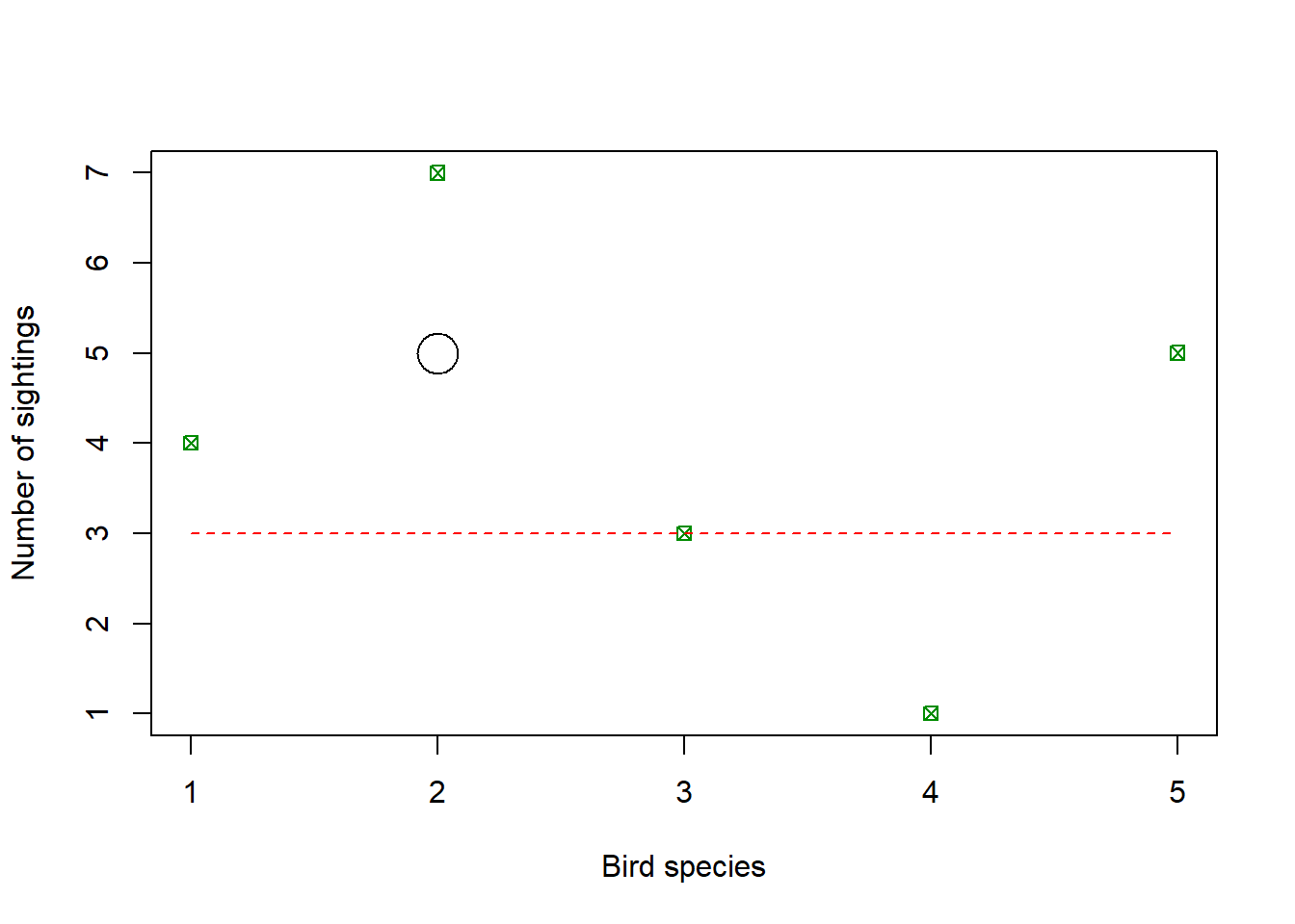

We have fully specified the relevant arguments of our plot function including the x and y variables, the labels, and the colour and style of the plotted points. Typing the name of each argument out in full means that it does not matter what order they are provided to the function in. You can try changing them around and re-running the code to see that there is no difference in the plot.

Code

#partial matching to create histogram
hist(w,fr=FALSE,br=5)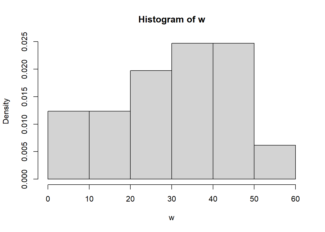

Specifying the arguments breaks and freq with br and fr is sufficient to distinguish them from the other possible arguments for the function hist(). This allows us to provide the values in any order without having to type out the entire argument names. However, the partial matching method requires awareness of any other possible arguments that could be matched and therefore how specific we have to be.

Code

#position matching to view first entries of object
head(y,4)

  Number       Bird   Size Seen
1      1        Tui  Large    4
2      2    Fantail  Small    7
3      3     WaxEye  Small    3
4      4 Kingfisher Medium    1

Code

#position matching to view last entries of object
tail(y,4)

  Number       Bird   Size Seen
2      2    Fantail  Small    7
3      3     WaxEye  Small    3
4      4 Kingfisher Medium    1
5      5   Bellbird Medium    5

If we can remember the order of arguments in the function head(), it is not necessary to specify head(x=y,n=4) to print the first 4 rows of the data frame y. Instead, if we enter the relevant values in the correct order, the function assigns them to be equal to arguments x and n respectively anyway.

Packages

Packages are collections of functions that have been developed to perform different types of analysis in R. Some packages come pre-installed when you download R, such as base, stats and graphics. These packages contain most of the functions you will need for completing these lessons.

In addition to the default R packages, new packages are continuously being developed and made available for more specific purposes. We will need to use some of them.

New packages are installed using the command install.packages(" "). An example is shown below.

Code

install.packages("readxl")

It is only necessary to install a package once. However, each time you use the package in a new session (or a new Markdown script) you can load it using library().

Code

library("readxl")

The Packages tab shows the packages you have installed. Packages can also be loaded by checking the box next to the package name.

Getting Help

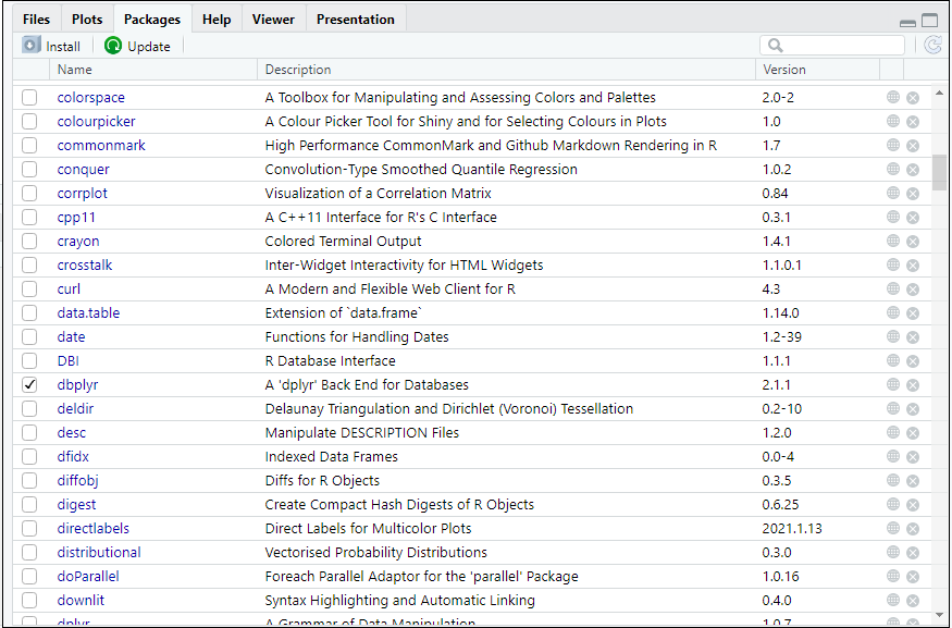
You can access the help file for any function in packages you have installed using ? followed by the function name

Code

?median

Even if the function is not in an installed package, you can find its help file with ??

Code

??read_xls

Alternatively, you can access the same files by navigating to the Help tab in the bottom right window and using the search bar.

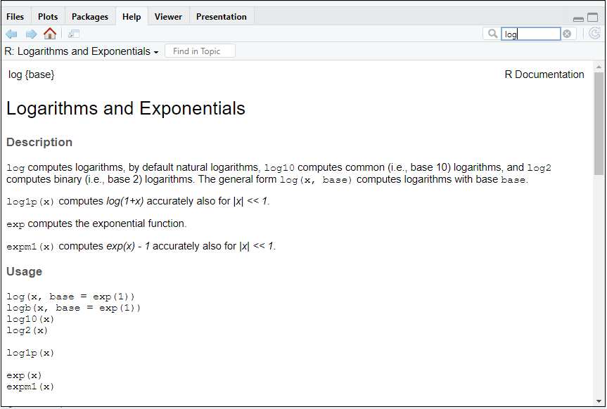
Sometimes the help files can be difficult to understand, so you can also try an Internet search of R along with the function name/argument e.g. “col argument in plot in R”. There are often step by step explanations and examples available.

If you want to carry out a particular operation, but are not sure which R functions to use for this, you can search your query directly to find ideas of things to try e.g. “How to make a box plot in R?”