18 Iron Deficiency

Low iron levels in infants and toddlers is a major health problem in New Zealand. This lesson investigates the prevalence of iron deficiency in sample data collected from three New Zealand cities, and the influence of some other factors like sex and age on this prevalence. It is presented by Dr Elaine Ferguson (Department of Human Nutrition, University of Otago).

Data

Data Summary

323 observations

29 variables

Variable	Type	Information
ID	Categorical	Child ID, not used for analysis.
hb	Continuous	Haemoglobin (g/L).
mcv	Continuous	Mean cell volume (fL).
zpp	Continuous	Zinc protoporphyrin (umol/mol hb).
ferritin	Continuous	Ferritin (ug/l).
iron3	Binary	1 (iron deficiency anaemic, Stage 3), 0 (not iron deficiency anaemic).
iron2	Binary	1 (iron deficient without anaemia, Stage 2), 0 (not iron deficient without anaemia).
iron1	Binary	1 (depleted iron stores but without deficiency, Stage 1), 0 (not depleted iron stores but without deficiency).
ncrp10	Binary	1 (elevated C-reactive protein indicating infection), 0 (no elevated C-reactive protein).
age	Continuous	Years.
infant	Binary	1 (infant), 0 (toddler).
birthwt	Continuous	Grams.
bf	Binary	1 (currently breastfeeding), 0 (not currently breastfeeding).
premi	Binary	1 (born premature), 0 (not born premature).
curff	Binary	1 (currently formula feeding), 0 (not currently formula feeding).
sex	Binary	1 (girl), 0 (boy).
caucasia	Binary	1 (caucasian), 0 (not caucasian).
tertiary	Binary	1 (mother has tertiary education), 0 (mother does not have tertiary education).
lowincom	Binary	1 (income <$20,000 in 1998 & 1999), 0 (income not <$20,000 in 1998 & 1999).
hiincome	Binary	1 (income >$70,000 in 1998 & 1999), 0 (income not >$70,000 in 1998 & 1999).
medincom	Binary	1 (income $20,000 to $70,000 in 1998 & 1999), 0 (income $20,000 to $70,000 in 1998 & 1999).
smokers	Binary	1 (smoker(s) in household), 0 (no smoker(s) in household).
marital	Binary	1 (mother in permanent relationship), 0 (mother not in permanent relationship).
nkjall	Continuous	Estimated total average energy intake/day.
nfeall	Continuous	Estimated total average iron intake/day.
fibre	Continuous	Estimated total average fibre intake/day.
ca	Continuous	Estimated total average calcium intake/day.
vtc	Continuous	Estimated total average vitamin C intake/day.
milk500	Binary	1 (>500ml milk/day), 0 (<500ml milk/day).

There are 2 files associated with this presentation. The first contains the data you will need to complete the lesson tasks, and the second contains descriptions of the variables included in the data file.

Download Iron Data.xls

Download Iron Variables.xls

Video

Important Information

This lesson uses analysis techniques for both count (proportion) and continuous data. Most of these have been explored in previous lessons so the code is initially hidden. It is recommended you leave the tasks below until after you have worked through the other lessons. These tasks can then function as revision exercises to help you recall the relevant techniques.

Objectives

Learning Objectives

This lesson provides the opportunity to recall and practice analysis techniques that have been previously demonstrated.

Reinforcing skills and concepts seen in earlier lessons:

Data wrangling - read data, exclude values, new variables, transform variables.
Data consolidation - summarise, cross-tabulation, response by levels of predictor.
Confidence intervals, hypothesis tests - proportions, difference in proportions, difference in means.
Bootstrap confidence interval.
Plotting - box plots, bar plots, scatter plots, histograms.
Multiple linear regression, ANOVA.

Tasks

In the late 1990s, researchers from the University of Otago carried out a study to assess the prevalence of iron deficiency in 6-24 month old children in the South Island of New Zealand. Iron deficiency is associated with detrimental effects on the health, growth and development of children, so they were also interested in exploring which factors have an association with iron deficiency status. To investigate these issues, the food intake of 323 children from Christchurch, Dunedin and Invercargill were monitored, and blood samples and other measurements were taken from the children.

0. Read data

0a. Read in the data

First make sure you have installed the package readxl and set the working directory.

Load the data into R.

Important Information

Name your data iron for easier reference later.

The code has been hidden initially, so you can try to load the data yourself first before checking the solutions.

Code

#loads readxl package
library(readxl)

#loads the data file and names it iron
iron<-read_xls("Iron Data.xls") 

#view beginning of data frame
head(iron)

Code

#loads readxl package
library(readxl)

Warning: package 'readxl' was built under R version 4.2.2

Code

#loads the data file and names it iron
iron<-read_xls("Iron Data.xls") 

#view beginning of data frame
head(iron)

# A tibble: 6 × 29
     id    hb   mcv   zpp ferritin iron3 iron2 iron1 ncrp10   age infant birthwt
  <dbl> <dbl> <dbl> <dbl>    <dbl> <dbl> <dbl> <dbl>  <dbl> <dbl>  <dbl>   <dbl>
1   258   124    79    54     22.8     0     0     0      0  22.2      0    2870
2   328   107    80    40      8       0     0     1      0  24.4      0    4500
3   349   110    75    NA     NA      NA    NA    NA      0  24.9      0    3020
4   362   115    81    50     14       0     0     0      0  21.9      0    4410
5   390   110    73    48      6       0     1     0      0  21.4      0    4310
6   413    NA    NA    NA     NA      NA    NA    NA     NA  22.4      0    3620
# … with 17 more variables: bf <dbl>, premi <dbl>, curff <dbl>, girl <dbl>,
#   caucasia <dbl>, tertiary <dbl>, lowincom <dbl>, hincome <dbl>,
#   medincom <dbl>, smokers <dbl>, marital <dbl>, nkjall <dbl>, nfeall <dbl>,
#   fibre <dbl>, ca <dbl>, vtc <dbl>, milk500 <dbl>
# ℹ Use `colnames()` to see all variable names

This opens a large data frame containing blood measurement data from the children study, as well as additional information about the children and their parents. We can find a list of these variables, as well as a description of what they measure, in the “Iron Variables.xls” file.

0b. Format the data

In order to make later calculations more straightforward, create a new factor variable status that combines the indicators iron1, iron2 and iron3. This will allow us to analyse other variables according to iron status.

Code

#status=0 indicates normal, status=1 indicates depleted iron
#status=2 indicates stage 2 deficiency, status=3 indicates stage 3 deficiency
iron$status<-as.factor(iron$iron1+2*iron$iron2+3*iron$iron3)

Code

#status=0 indicates normal, status=1 indicates depleted iron
#status=2 indicates stage 2 deficiency, status=3 indicates stage 3 deficiency
iron$status<-as.factor(iron$iron1+2*iron$iron2+3*iron$iron3)

1. Data Summary, Proportions, Exclude NA’s

1a. Data Summary, Proportion Table

Four blood measurements were used to categorise the children as either Stage 1, 2 or 3 iron deficient, or as having normal iron levels.

Obtain summary statistics and proportions for the variable status which tell us how many children are in each group.

Code

#frequency
summary(iron$status)  

#proportions calculated from table 
prop.table(table(iron$status))

Code

#frequency
summary(iron$status)

   0    1    2    3 NA's 
 202   28   11    8   74

Code

#proportions calculated from table 
prop.table(table(iron$status))


         0          1          2          3 
0.81124498 0.11244980 0.04417671 0.03212851

The majority of child have normal iron levels, although 11% have stage 1 iron deficiency. Only a small proportion have stage 2 (4%) and stage 3 (3%) deficiency.

1b. Exclude NA’s

Some children have not been categorised into one of these groups, because they had missing blood sample measurements (NAs). We therefore want to exclude these cases from the analysis.

Code

 #includes only the rows (cases) with no NA's in a new data frame ironB
ironB<-iron[!is.na(iron$status),]

Code

 #includes only the rows (cases) with no NA's in a new data frame ironB
ironB<-iron[!is.na(iron$status),]

2. Data Summary, Exclude Values

The factor ncrp10 measures whether a child has elevated C-reactive protein levels, which indicates an infection. In such cases, iron status categorisation is unreliable.

Obtain statistics to tell us how many children have elevated C-reactive protein levels, then create a new data frame that excludes these children from the analysis.

Code

#number of children
nrow(ironB[ironB$ncrp10=="0",])
(ironB[ironB$ncrp10=="1",])

#remove elevated ncrp10
ironNC<-ironB[!(ironB$ncrp10=="1"),]

Code

#number of children
nrow(ironB[ironB$ncrp10=="0",])

[1] 233

Code

nrow(ironB[ironB$ncrp10=="1",])

[1] 16

Code

#remove elevated ncrp10
ironNC<-ironB[!(ironB$ncrp10=="1"),]

16 out of 249 children sampled had elevated C-reactive protein levels.

3. Confidence Intervals (proportions)

Calculate 95% confidence intervals (using R) for the proportion of children with each level of status.

What do you conclude from your confidence intervals?

Code

#first argument is the number of successes (in this case having a particular iron status)
#second argument is number of trials
prop.test(length(which(ironNC$status=="0")),n=length(ironNC$status))

Repeat for all levels of status.

Code

#first argument is the number of successes (in this case having a particular iron status)
#second argument is number of trials
prop.test(length(which(ironNC$status=="0")),n=length(ironNC$status))


    1-sample proportions test with continuity correction

data:  length(which(ironNC$status == "0")) out of length(ironNC$status), null probability 0.5
X-squared = 81.734, df = 1, p-value < 2.2e-16
alternative hypothesis: true p is not equal to 0.5
95 percent confidence interval:
 0.7398021 0.8466904
sample estimates:
        p 
0.7982833

Code

prop.test(length(which(ironNC$status=="1")),n=length(ironNC$status))


    1-sample proportions test with continuity correction

data:  length(which(ironNC$status == "1")) out of length(ironNC$status), null probability 0.5
X-squared = 132.94, df = 1, p-value < 2.2e-16
alternative hypothesis: true p is not equal to 0.5
95 percent confidence interval:
 0.08266681 0.17061914
sample estimates:
        p 
0.1201717

Code

prop.test(length(which(ironNC$status=="2")),n=length(ironNC$status))


    1-sample proportions test with continuity correction

data:  length(which(ironNC$status == "2")) out of length(ironNC$status), null probability 0.5
X-squared = 189.27, df = 1, p-value < 2.2e-16
alternative hypothesis: true p is not equal to 0.5
95 percent confidence interval:
 0.02501273 0.08520400
sample estimates:
        p 
0.0472103

Code

prop.test(length(which(ironNC$status=="3")),n=length(ironNC$status))


    1-sample proportions test with continuity correction

data:  length(which(ironNC$status == "3")) out of length(ironNC$status), null probability 0.5
X-squared = 200.24, df = 1, p-value < 2.2e-16
alternative hypothesis: true p is not equal to 0.5
95 percent confidence interval:
 0.01605194 0.06903145
sample estimates:
         p 
0.03433476

We can be 95% confident that the true proportion of children with normal iron levels is between 0.7398 0.8467.For stage 1 deficiency the true proportion is between 0.08267 and 0.1706. For stage 2 we can be 95% confident that the actual population proportion is between 0.0250 and 0.0852. Stage 3 is the least common, with a true proportion between 0.0161 and 0.0690.

4. Cross-Tabulation, Bar Plot, Box Plot, Confidence Intervals (difference in proportions)

4a. Cross-Tabulation

To investigate whether the prevalence of iron deficiency varies with age, create a contingency table of the variables status and infant.

Code

table(ironNC$status,ironNC$infant,dnn=c("Iron level","Infant"))

Code

table(ironNC$status,ironNC$infant,dnn=c("Iron level","Infant"))

          Infant
Iron level   0   1
         0 123  63
         1  25   3
         2   9   2
         3   4   4

4b. Bar Plot

A nice way to display these results visually is a bar chart.

What differences do you notice between the counts of children with each iron status, based on this graph?

Construct table of values

Code

#construct table without labels to supply heights to bars
ironMatrix<-table(ironNC$status,ironNC$infant)

Produce bar plot with legend

Code

#bar plot
barplot(ironMatrix,beside=TRUE,names.arg=c("Toddler","Infant"),col=rep(c("orchid4","orchid2","orange1","darkorange3"),2),ylab="Count",xlab="Age",
  main="Iron level by Age")

#legend
legend("topright",c("Normal","Depleted","Stage 2", "Stage 3"),fill=c("orchid4","orchid2","orange1","darkorange3"))

Code

#construct table without labels to supply heights to bars
ironMatrix<-table(ironNC$status,ironNC$infant)

Code

#bar plot
barplot(ironMatrix,beside=TRUE,names.arg=c("Toddler","Infant"),col=rep(c("orchid4","orchid2","orange1","darkorange3"),2),ylab="Count",xlab="Age",
  main="Iron level by Age")

#legend
legend("topright",c("Normal","Depleted","Stage 2", "Stage 3"),fill=c("orchid4","orchid2","orange1","darkorange3"))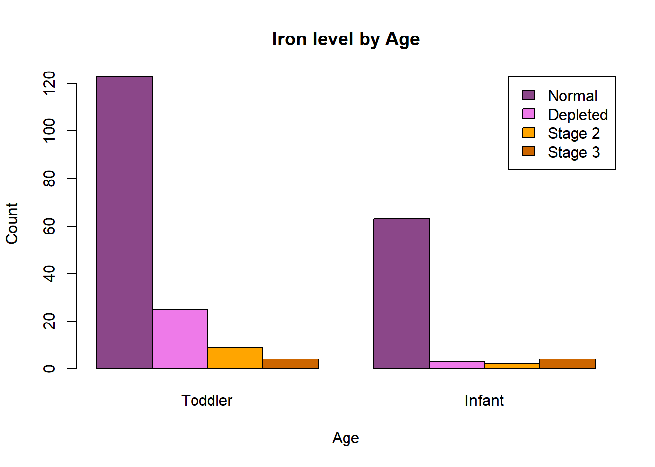

There are more observations overall for toddlers than infants. Toddlers have higher levels of stage 1 and stage 2 iron deficiency relative to normal iron levels than infants. There were a similar number of infants as toddlers with stage 3 iron deficiency, although this represents a greater proportion of infants so it appears stage 3 deficiency is more common at this age.

4c. Box Plot

We can create a box-and-whiskers plot to show how the continuous variable age varies by iron status.

Code

boxplot(age~status,data=ironNC,xlab="Iron deficiency status",ylab="Age (months)")

Code

boxplot(age~status,data=ironNC,xlab="Iron deficiency status",ylab="Age (months)")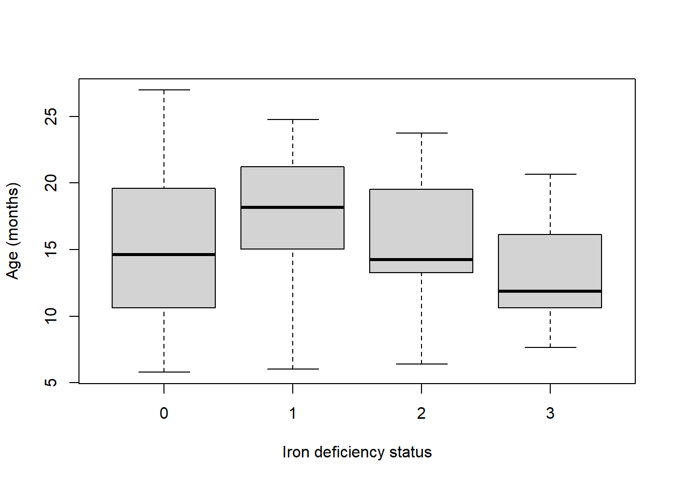

There is considerable overlap between the age distributions of children with different iron statuses. For normal iron status the variability in age is the greatest, this is unsurprising as this category also has the highest number of children. Children with stage 3 iron deficiency tend to be slightly younger with a median age of approximately 11 months. Children with stage 1 deficiency tend to be older with a median age of around 18 months.

4d. Proportions

Display a summary table of status by infant (age indicator) using percentages instead of counts

Code

#margin=2 indicates we are interested in the proportion of each iron status for infants and toddlers
prop.table(table(ironNC$status,ironNC$infant,dnn=c("Iron Status","Infant")),margin=2)

Code

#margin=2 indicates we are interested in the proportion of each iron status for infants and toddlers
 prop.table(table(ironNC$status,ironNC$infant,dnn=c("Iron Status","Infant")),margin=2)

           Infant
Iron Status          0          1
          0 0.76397516 0.87500000
          1 0.15527950 0.04166667
          2 0.05590062 0.02777778
          3 0.02484472 0.05555556

This tells us that, for example, 76.4% of toddlers (ages 12 to 24 months) had normal iron status, compared to 87.5% of infants (ages 6 to 11.9 months).

4e. Confidence Interval (difference in proportions)

Calculate 95% confidence intervals for the difference in proportions of toddlers and infants who have each status of iron deficiency (normal=0, depleted=1, Stage 2=2 and Stage 3=3).

What do you conclude from your confidence intervals?

This code shows the calculation procedure for normal iron status.

Code

#First argument is a vector of successes for each of the groups to be compared, interested in proportion of infants vs toddlers with normal iron status
#second argument is a vector of the number of trials for each group

prop.test(c(length(which(ironNC$infant=="1"&ironNC$status=="0")),length(which(ironNC$infant=="0"&ironNC$status=="0"))),
  n=c(length(which(ironNC$infant=="1")),length(which(ironNC$infant=="0"))))

Modify this code to calculate the difference in proportions for depleted, Stage 2 deficiency, and Stage 3 deficiency iron status.

Code

#First argument is a vector of successes for each of the groups to be compared, interested in proportion of infants vs toddlers with normal iron status
#second argument is a vector of the number of trials for each group

prop.test(c(length(which(ironNC$infant=="1"&ironNC$status=="0")),length(which(ironNC$infant=="0"&ironNC$status=="0"))),
  n=c(length(which(ironNC$infant=="1")),length(which(ironNC$infant=="0"))))


    2-sample test for equality of proportions with continuity correction

data:  c(length(which(ironNC$infant == "1" & ironNC$status == "0")), length(which(ironNC$infant == "0" & ironNC$status == "0"))) out of c(length(which(ironNC$infant == "1")), length(which(ironNC$infant == "0")))
X-squared = 3.1501, df = 1, p-value = 0.07592
alternative hypothesis: two.sided
95 percent confidence interval:
 0.0002875989 0.2217620906
sample estimates:
   prop 1    prop 2 
0.8750000 0.7639752

Code

#First argument is a vector of successes for each of the groups to be compared, interested in proportion of infants vs toddlers with depleted iron status
#second argument is a vector of the number of trials for each group

prop.test(c(length(which(ironNC$infant=="1"&ironNC$status=="1")),length(which(ironNC$infant=="0"&ironNC$status=="1"))),
  n=c(length(which(ironNC$infant=="1")),length(which(ironNC$infant=="0"))))


    2-sample test for equality of proportions with continuity correction

data:  c(length(which(ironNC$infant == "1" & ironNC$status == "1")), length(which(ironNC$infant == "0" & ironNC$status == "1"))) out of c(length(which(ironNC$infant == "1")), length(which(ironNC$infant == "0")))
X-squared = 5.0467, df = 1, p-value = 0.02467
alternative hypothesis: two.sided
95 percent confidence interval:
 -0.19618942 -0.03103625
sample estimates:
    prop 1     prop 2 
0.04166667 0.15527950

Code

#First argument is a vector of successes for each of the groups to be compared, interested in proportion of infants vs toddlers with stage 2 deficiency iron status
#second argument is a vector of the number of trials for each group

prop.test(c(length(which(ironNC$infant=="1"&ironNC$status=="2")),length(which(ironNC$infant=="0"&ironNC$status=="2"))),
  n=c(length(which(ironNC$infant=="1")),length(which(ironNC$infant=="0"))))

Warning in prop.test(c(length(which(ironNC$infant == "1" & ironNC$status == :
Chi-squared approximation may be incorrect


    2-sample test for equality of proportions with continuity correction

data:  c(length(which(ironNC$infant == "1" & ironNC$status == "2")), length(which(ironNC$infant == "0" & ironNC$status == "2"))) out of c(length(which(ironNC$infant == "1")), length(which(ironNC$infant == "0")))
X-squared = 0.36126, df = 1, p-value = 0.5478
alternative hypothesis: two.sided
95 percent confidence interval:
 -0.09013541  0.03388973
sample estimates:
    prop 1     prop 2 
0.02777778 0.05590062

Code

#First argument is a vector of successes for each of the groups to be compared, interested in proportion of infants vs toddlers with stage 3 deficiency iron status
#second argument is a vector of the number of trials for each group

prop.test(c(length(which(ironNC$infant=="1"&ironNC$status=="3")),length(which(ironNC$infant=="0"&ironNC$status=="3"))),
  n=c(length(which(ironNC$infant=="1")),length(which(ironNC$infant=="0"))))

Warning in prop.test(c(length(which(ironNC$infant == "1" & ironNC$status == :
Chi-squared approximation may be incorrect


    2-sample test for equality of proportions with continuity correction

data:  c(length(which(ironNC$infant == "1" & ironNC$status == "3")), length(which(ironNC$infant == "0" & ironNC$status == "3"))) out of c(length(which(ironNC$infant == "1")), length(which(ironNC$infant == "0")))
X-squared = 0.64052, df = 1, p-value = 0.4235
alternative hypothesis: two.sided
95 percent confidence interval:
 -0.03745532  0.09887699
sample estimates:
    prop 1     prop 2 
0.05555556 0.02484472

There is a borderline significant difference in the proportion of infants and toddlers with normal iron status. The p-value is 0.0759, indicating there is not enough evidence to reject the null hypothesis of no difference. However, the 95% confidence interval for the difference is from 0.0003 to 0.2218, indicating there is a positive true difference in proportion of infants and toddlers with normal iron levels.

There is significant evidence that the proportion of infants with stage 1 iron deficiency is less than the proportion of toddlers. The p-value is 0.0247, and the confidence interval for the true difference in proportions is entirely negative from -0.1962 to -0.0310.

As the respective p-values are greater than 0.05 and the confidence intervals for the true difference in proportions include both positive and negative values, there is no significant evidence of a difference between the proportion of infants and toddlers with stage 2 or stage 3 iron deficiency.

5. Extension: Cross-Tabulation, Bar Plot, Box Plot, Confidence Intervals (difference in proportions)

Extension

Investigate the effect of some of the other factors in the spreadsheet on iron deficiency status, using techniques from earlier tasks (tables, bar plots, box plots, confidence intervals).

For example, you could look at whether the sex (girl) of the child has an effect on their iron intake, or whether prematurely born (premi) babies were more likely to be iron deficient.

6. Normality Check, Transformation

The variables hb, mcv, zpp and ferritin are measurements taken from the blood samples of the children in the study, measuring haemoglobin levels, cell volume, zinc levels and iron levels.

Check the distributions of these readings for normality by creating histograms.

Code

#change breaks= to see distribution
hist(ironNC$hb,xlab="Haemoglobin level",main="Histogram of Haemoglobin levels",breaks=10)

Plot the other three histograms, and comment on the normality of the data. If the data are not normally distributed, suggest a way of transforming the data that may remedy this problem, and investigate whether this transformation offers an improvement.

Code

#change breaks= to see distribution
hist(ironNC$hb,xlab="Haemoglobin level",main="Histogram of Haemoglobin levels",breaks=10)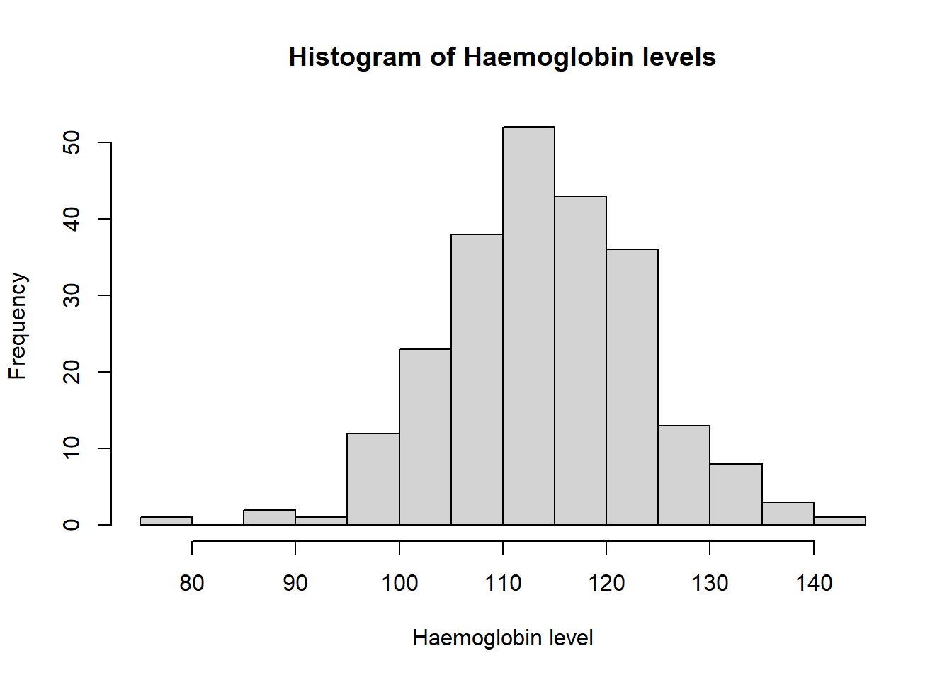

Code

hist(ironNC$mcv,xlab="Mean Cell Volume",main="Histogram of Mean Cell Volumes",breaks=10)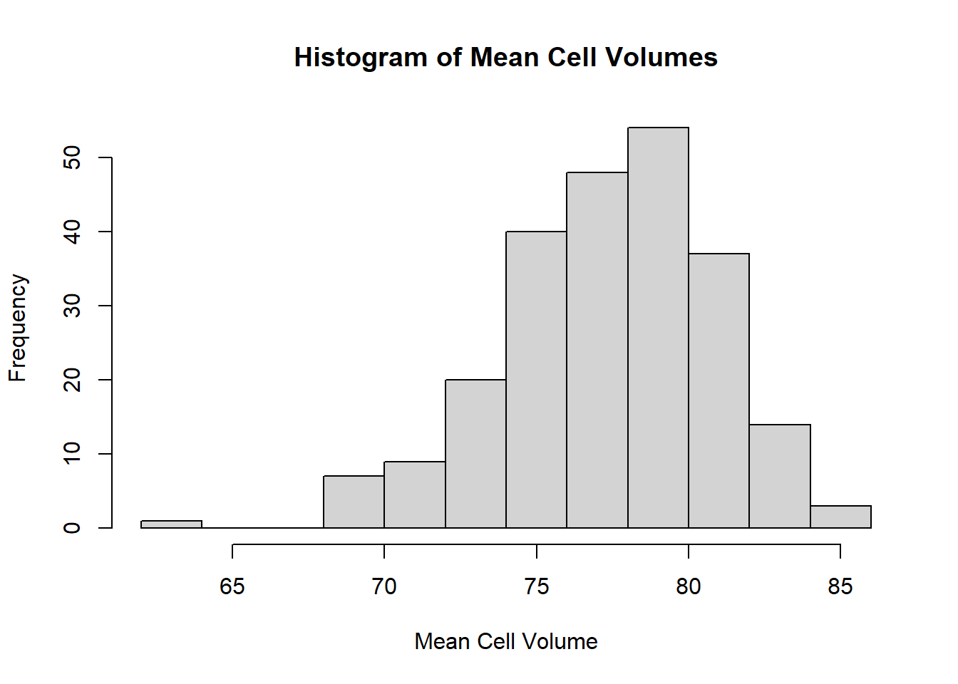

Code

hist(ironNC$zpp,xlab="Zinc Protoporphyrin",main="Histogram of Zinc Protoporphyrin",breaks=10)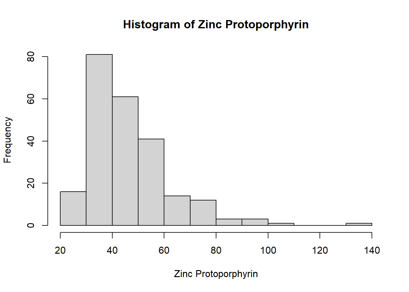

Code

hist(ironNC$ferritin,xlab="Ferritin level",main="Histogram of Ferritin levels",breaks=10)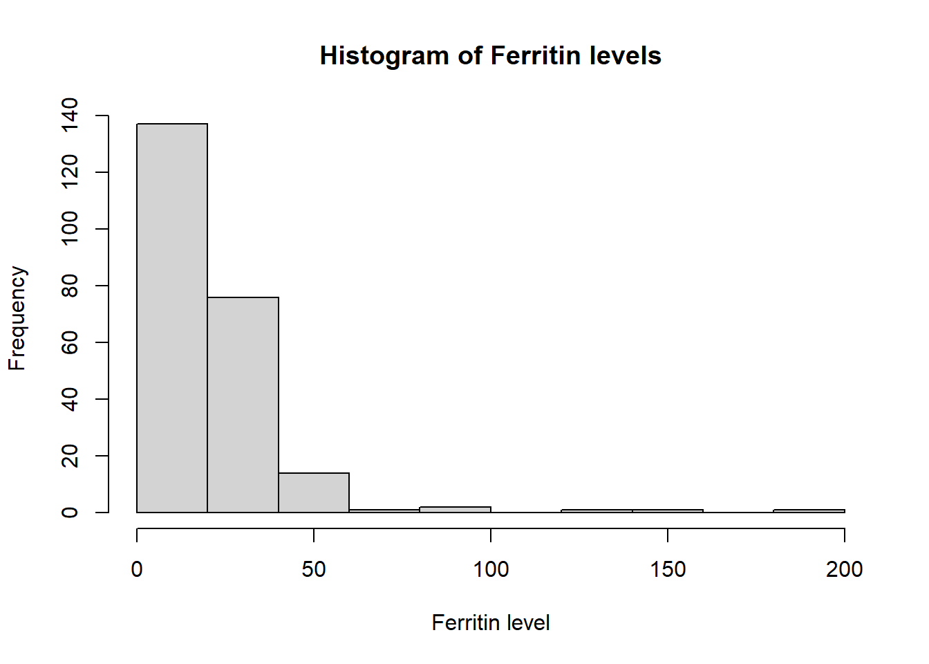

Haemoglobin appears to be normally distributed. The histograms of mean cell volume, zinc protoporphyrin and ferritin are highly skewed. A log transformation of the values may result in a normal distribution.

7. Summary Statistics, Box Plot, Confidence Interval, Hypothesis Test (difference in means)

The variable ferritin measures iron stores in the blood.

Investigate the effect of breast feeding (bf) on this variable. Calculate some informative summary statistics, produce a box plot, construct a 95% confidence interval and perform a hypothesis test.

Based on these results, does there appear to be a difference in iron stores for the breast fed children compared to the other children?

Summary statistics

Code

#number of observations
tapply(ironNC$ferritin,INDEX=ironNC$bf,FUN=length)

#mean
tapply(ironNC$ferritin,INDEX=ironNC$bf,FUN=mean)

#standard deviation
tapply(ironNC$ferritin,INDEX=ironNC$bf,FUN=sd)

Box plot

Code

ferritinBox<-boxplot(ironNC$ferritin~ironNC$bf,xlab="Breastfeeding
(1=breastfed)",ylab="Ferritin",main="Ferritin level by Breastfeeding status")

#prints the value of outliers on the plot
ferritinBox$out

Confidence interval, hypothesis test for difference in means

Code

#first test if variances are equal
var.test(ferritin ~ bf, data=ironNC, alternative = "two.sided") 

#significant evidence against null hypothesis that variances are equal, use var.equal=F in t test
t.test(ironNC$ferritin[ironNC$bf=="0"],ironNC$ferritin[ironNC$bf=="1"],var.equal = FALSE)

Summary statistics

Code

#number of observations
tapply(ironNC$ferritin,INDEX=ironNC$bf,FUN=length)

  0   1 
179  54

Code

#mean
tapply(ironNC$ferritin,INDEX=ironNC$bf,FUN=mean)

       0        1 
19.99358 30.07407

Code

#standard deviation
tapply(ironNC$ferritin,INDEX=ironNC$bf,FUN=sd)

       0        1 
13.70458 32.71092

There were more than 3 times as many bottle fed children in the study as those that were breast fed. Breast fed children had a higher mean ferritin level, but also more variation around this mean with a larger standard deviation in ferritin values.

Box plot

Code

ferritinBox<-boxplot(ironNC$ferritin~ironNC$bf,xlab="Breastfeeding
(1=breastfed)",ylab="Ferritin",main="Ferritin level by Breastfeeding status")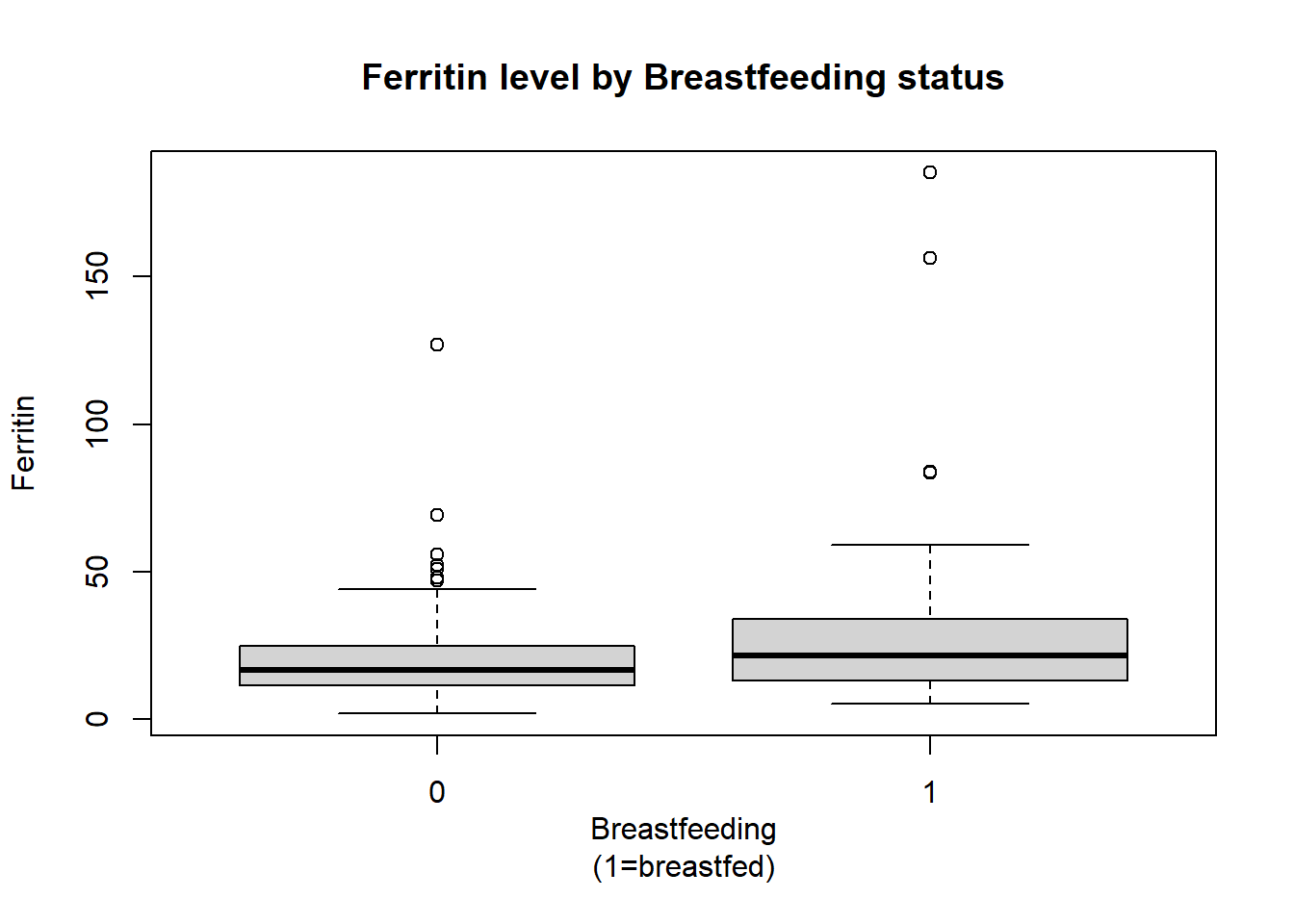

Code

#prints the value of outliers on the plot
ferritinBox$out

 [1]  52.1  47.9  69.2  50.9  55.8 126.9  47.0  83.6  83.8 185.1 156.3

These box plots show that there is some overlap between the middle 50% of ferritin values of bottle and breast fed children, although 75% of the ferritin values for bottle fed children are less than the median ferritin value for breast fed children. There are more observations classified as outliers in the bottle fed group.

Code

#first test if variances are equal
var.test(ferritin ~ bf, data=ironNC, alternative = "two.sided")


    F test to compare two variances

data:  ferritin by bf
F = 0.17553, num df = 178, denom df = 53, p-value < 2.2e-16
alternative hypothesis: true ratio of variances is not equal to 1
95 percent confidence interval:
 0.1104173 0.2648368
sample estimates:
ratio of variances 
         0.1755277

Code

#significant evidence against null hypothesis that variances are equal, use var.equal=F in t test
t.test(ironNC$ferritin[ironNC$bf=="0"],ironNC$ferritin[ironNC$bf=="1"],var.equal = FALSE)


    Welch Two Sample t-test

data:  ironNC$ferritin[ironNC$bf == "0"] and ironNC$ferritin[ironNC$bf == "1"]
t = -2.2069, df = 58.713, p-value = 0.03124
alternative hypothesis: true difference in means is not equal to 0
95 percent confidence interval:
 -19.2214397  -0.9395576
sample estimates:
mean of x mean of y 
 19.99358  30.07407

The p-value of 0.0312 indicates significant evidence of a true difference in mean ferritin levels between bottle and breast fed children. We can be 95% confident the true difference in means is between -19.2214 and -0.9396, therefore can conclude children who were breast fed have higher mean ferritin levels than those who were bottle fed.

Repeat this process with the predictor variables formula feeding (curff) and high cow’s milk intake (milk500) and report your conclusions.

8. Bootstrap, Histogram (difference in means)

Estimate the distribution of the mean difference in iron stores (ferritin) between children who were not breast fed and those who were (bf), and using this distribution provide a new estimate of the mean difference along with a 95% confidence interval it.

Important Information

To construct such a distribution, we use the bootstrap technique. This involves randomly sampling a new data set from the original sampled data. By doing this several times, we create a large number of data sets that we might have seen had we performed the experiment multiple times. By computing the mean for each of these data sets, we get an estimate of the distribution of the statistic.

Have a look at previous lessons for examples of how to write a function and bootstrap using boot(), and plot the results.

What do you conclude from your bootstrap confidence interval for the difference in the means?

Bootstrap

Code

#set seed so you get the same results when running again
set.seed(8)  

library(boot)

 #function that calculates the difference in means from the bootstrapped samples
meandiffFun<-function(data,indices){ 
   data1<-data[data$bf=="0",]
  dataInd1<-data1[indices,]
  data2<-data[data$bf=="1",]
  dataInd2<-data2[indices,]
  meandiff<-mean(dataInd1$ferritin,na.rm=T)-mean(dataInd2$ferritin,na.rm=T)
  return(meandiff)
}

 #bootstrap difference in mean ferritin levels between children who were and were not breastfed
#create object called meandiffBoot with the output of the bootstrapping procedure
meandiffBoot<-boot(ironNC,statistic=meandiffFun, R=10000)

View summary statistics of the results by calling the object.

Code

meandiffBoot

Calculate a 95% confidence interval.

Code

#your standard error numbers will be slightly different
lower<--10.0805-1.96*4.603457
upper<--10.0805+1.96*4.603457

Graph showing the distribution of the mean of the bootstrap samples with a density curve and 95% confidence interval limits plotted on top.

Code

#plot density histogram of bootstrap results
hist(meandiffBoot$t,breaks=20,freq=F,xlab="Difference in Mean Iron Stores", 
  main="Difference in Mean Iron Stores \n between Non-Breastfed and Breastfed Children") 

 #add a smoothed line to show the distribution
lines(density(meandiffBoot$t,na.rm=T), lwd = 2, col = "royalblue1")

#95% ci limits
abline(v=c(lower,upper),lty=2,col="royalblue4")

Code

#set seed so you get the same results when running again
set.seed(8)  

library(boot)

Warning: package 'boot' was built under R version 4.2.2

Code

 #function that calculates the difference in means from the bootstrapped samples
meandiffFun<-function(data,indices){ 
   data1<-data[data$bf=="0",]
  dataInd1<-data1[indices,]
  data2<-data[data$bf=="1",]
  dataInd2<-data2[indices,]
  meandiff<-mean(dataInd1$ferritin,na.rm=T)-mean(dataInd2$ferritin,na.rm=T)
  return(meandiff)
}

 #bootstrap difference in mean ferritin levels between children who were and were not breastfed
#create object called meandiffBoot with the output of the bootstrapping procedure
meandiffBoot<-boot(ironNC,statistic=meandiffFun, R=10000)

Code

meandiffBoot


ORDINARY NONPARAMETRIC BOOTSTRAP


Call:
boot(data = ironNC, statistic = meandiffFun, R = 10000)


Bootstrap Statistics :
    original      bias    std. error
t1* -10.0805 -0.03968669     4.51293

Code

#your standard error numbers will be slightly different
lower<--10.0805-1.96*4.603457
upper<--10.0805+1.96*4.603457

Code

#plot density histogram of bootstrap results
hist(meandiffBoot$t,breaks=20,freq=FALSE,xlab="Difference in Mean Iron Stores", 
  main="Difference in Mean Iron Stores \n between Non-Breastfed and Breastfed Children") 

 #add a smoothed line to show the distribution
lines(density(meandiffBoot$t,na.rm=T), lwd = 2, col = "royalblue1")

#95% ci limits
abline(v=c(lower,upper),lty=2,col="royalblue4")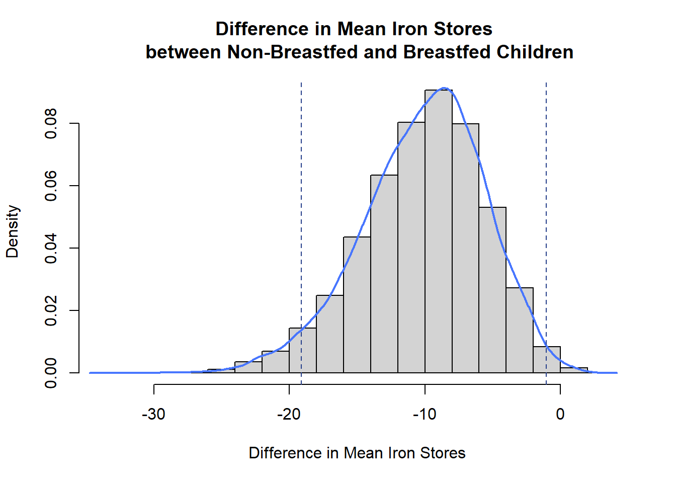

The bootstrapped difference in means follows a near normal distribution around a mean of -10.0805 with left skew (left side tail). This mean of means matches the difference in ferritin means of the bottle and breast fed children we calculated earlier, and the distribution of bootstrapped difference in mean estimates around it give an indication of the amount of variability in our estimate due to sampling.

The bootstrap confidence interval is slightly narrower than the one calculated earlier and includes only negative values so leads to the same conclusion. There is significant evidence to conclude a difference in mean ferritin levels between bottle and breast fed children.

Perform a bootstrap for the mean difference in iron stores for formula fed children and other children (curff), and report your findings.

9.Log-Transformation, Scatter Plots, Correlation

Now use correlations to examine the relationships between some of the continuous variables and the iron stores.

9a. Log-Transformation

From earlier, you should have found that the distribution of the ferritin data is skewed.

Construct a new variable, the log transformed ferritin levels, that follows a normal distribution.

Plot a histogram of nfeall, the dietary iron data, to determine whether a transformation is necessary for this data too. If it is, add a log transformed nfeall variable to the ironNC data frame.

Code

#log ferritin
ironNC$logferritin<-log(ironNC$ferritin)

Code

hist(ironNC$nfeall)

#log nfeall
ironNC$lognfeall<-log(ironNC$nfeall)

Code

#log ferritin
ironNC$logferritin<-log(ironNC$ferritin)

Code

hist(ironNC$nfeall)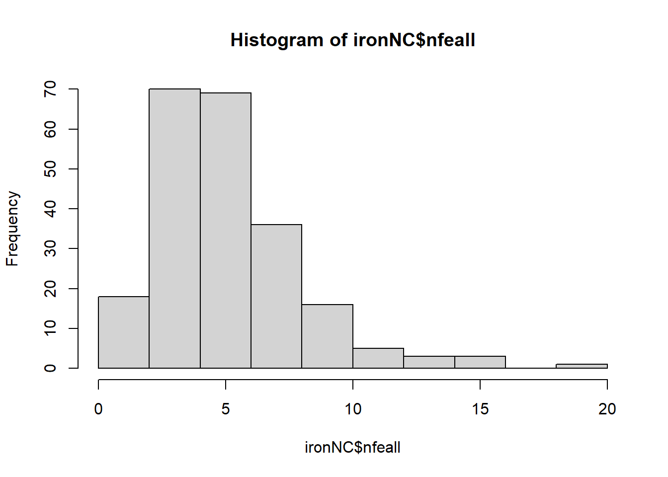

Code

#log nfeall
ironNC$lognfeall<-log(ironNC$nfeall)

The distribution of dietary iron is right skewed, so should also be log transformed.

9b. Scatter Plot

Produce a scatter plot of the two variables, entering logferritin and lognfeall as the variates.

Based on the graph, does there appear to be a relationship between the two variables? If so, what is the relationship?

Code

plot(ironNC$lognfeall,ironNC$logferritin,ylab="log(Ferritin)",xlab="log(Dietry Iron)",pch=4)

Code

plot(ironNC$lognfeall,ironNC$logferritin,ylab="log(Ferritin)",xlab="log(Dietry Iron)",pch=4)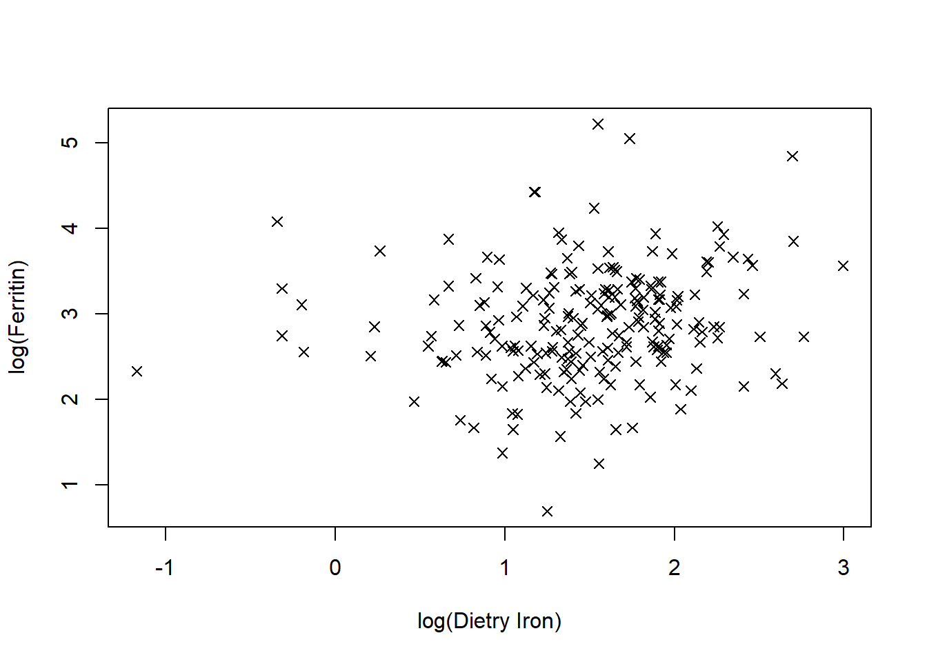

There appears to be a weak positive relationship. As log dietary iron increases so does log ferritin, although there is quite a lot of variation in individual values.

9c. Correlation

We can test to see if the relationship is significant using the correlation between the two variables using cor.test().

Have a look at the help file for this function, then use it to test the correlation between your log ferritin and log nfeall variables.

If the p-value from the hypothesis test is less than 0.05, there is a significant relationship between the two variables. Is that the case here?

Code

cor.test(ironNC$logferritin,ironNC$lognfeall)

Code

cor.test(ironNC$logferritin,ironNC$lognfeall)


    Pearson's product-moment correlation

data:  ironNC$logferritin and ironNC$lognfeall
t = 2.3578, df = 219, p-value = 0.01926
alternative hypothesis: true correlation is not equal to 0
95 percent confidence interval:
 0.02590874 0.28342798
sample estimates:
     cor 
0.157342

The p-value is 0.0193, indicating there is significant evidence of a non-zero correlation between log ferritin and log dietary iron. The 95% confidence interval is for a (positive) correlation of between 0.0259 and 0.2834, with a best estimate of 0.1573.

9d. Extension: Log-Transformation, Scatter Plots, Correlation

Extension

Explore the relationship between (log) iron stores and some of the other continuous variables, e.g. dietary fibre (fibre), using log-transforms where necessary. Report your findings.

10. Multiple Linear Regression, ANOVA

Return to the original iron data set, as we want to now include children with elevated nrcp10 in our analysis (and see how it affects iron).

The variables girl and premi are actually factors, so recode them as such. Also add the log transformed ferritin and nfeall to this data set. Then fit and interpret a linear model with logferritin as the response, and age+lognfeall+premi+ncrp10+girl as the explanatory variables.

Convert relevant variables to factors

Code

iron$girl<-as.factor(iron$girl)
iron$premi<-as.factor(iron$premi)
iron$ncrp10<-as.factor(iron$ncrp10)
iron$logferritin<-log(iron$ferritin)
iron$lognfeall<-log(iron$nfeall)

Linear model, ANOVA

Code

ironModel<-lm(logferritin~age+lognfeall+ncrp10+premi+girl,data=iron)

#model parameters
summary(ironModel)

#anova
anova(ironModel)

Code

iron$girl<-as.factor(iron$girl)
iron$premi<-as.factor(iron$premi)
iron$ncrp10<-as.factor(iron$ncrp10)
iron$logferritin<-log(iron$ferritin)
iron$lognfeall<-log(iron$nfeall)

Code

ironModel<-lm(logferritin~age+lognfeall+ncrp10+premi+girl,data=iron)

#model parameters
summary(ironModel)


Call:
lm(formula = logferritin ~ age + lognfeall + ncrp10 + premi + 
    girl, data = iron)

Residuals:
     Min       1Q   Median       3Q      Max 
-1.75984 -0.38953  0.01345  0.39084  1.94650 

Coefficients:
             Estimate Std. Error t value Pr(>|t|)    
(Intercept)  3.103894   0.167266  18.557  < 2e-16 ***
age         -0.030467   0.007556  -4.032 7.49e-05 ***
lognfeall    0.147865   0.067629   2.186   0.0298 *  
ncrp101      0.794171   0.165461   4.800 2.83e-06 ***
premi1      -0.205973   0.112545  -1.830   0.0685 .  
girl1        0.155856   0.080282   1.941   0.0534 .  
---
Signif. codes:  0 '***' 0.001 '**' 0.01 '*' 0.05 '.' 0.1 ' ' 1

Residual standard error: 0.6133 on 234 degrees of freedom
  (83 observations deleted due to missingness)
Multiple R-squared:  0.184, Adjusted R-squared:  0.1666 
F-statistic: 10.56 on 5 and 234 DF,  p-value: 3.732e-09

Code

#anova
anova(ironModel)

Analysis of Variance Table

Response: logferritin
           Df Sum Sq Mean Sq F value    Pr(>F)    
age         1  5.555  5.5552 14.7707 0.0001565 ***
lognfeall   1  3.383  3.3833  8.9958 0.0029984 ** 
ncrp10      1  8.262  8.2624 21.9689 4.706e-06 ***
premi       1  1.233  1.2327  3.2777 0.0715117 .  
girl        1  1.417  1.4175  3.7689 0.0534160 .  
Residuals 234 88.007  0.3761                      
---
Signif. codes:  0 '***' 0.001 '**' 0.01 '*' 0.05 '.' 0.1 ' ' 1

Code

#residuals
plot(ironModel)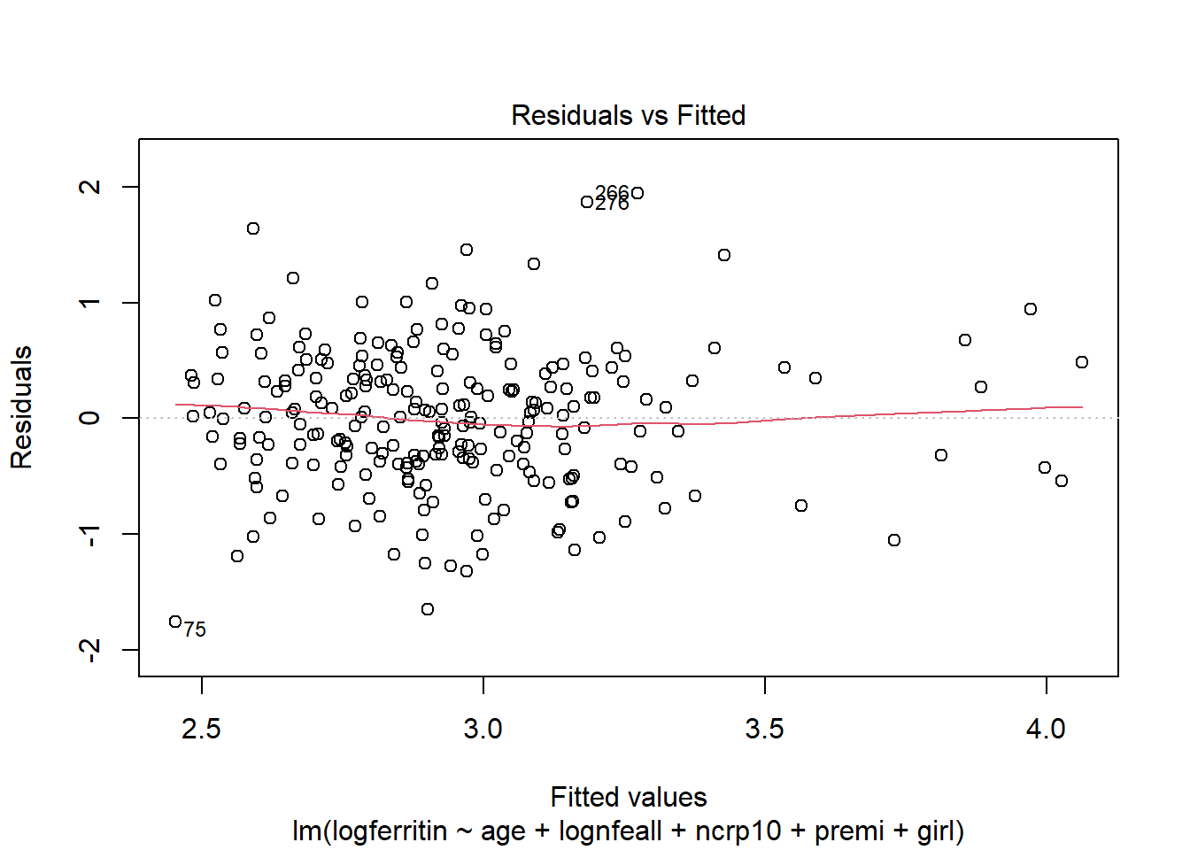

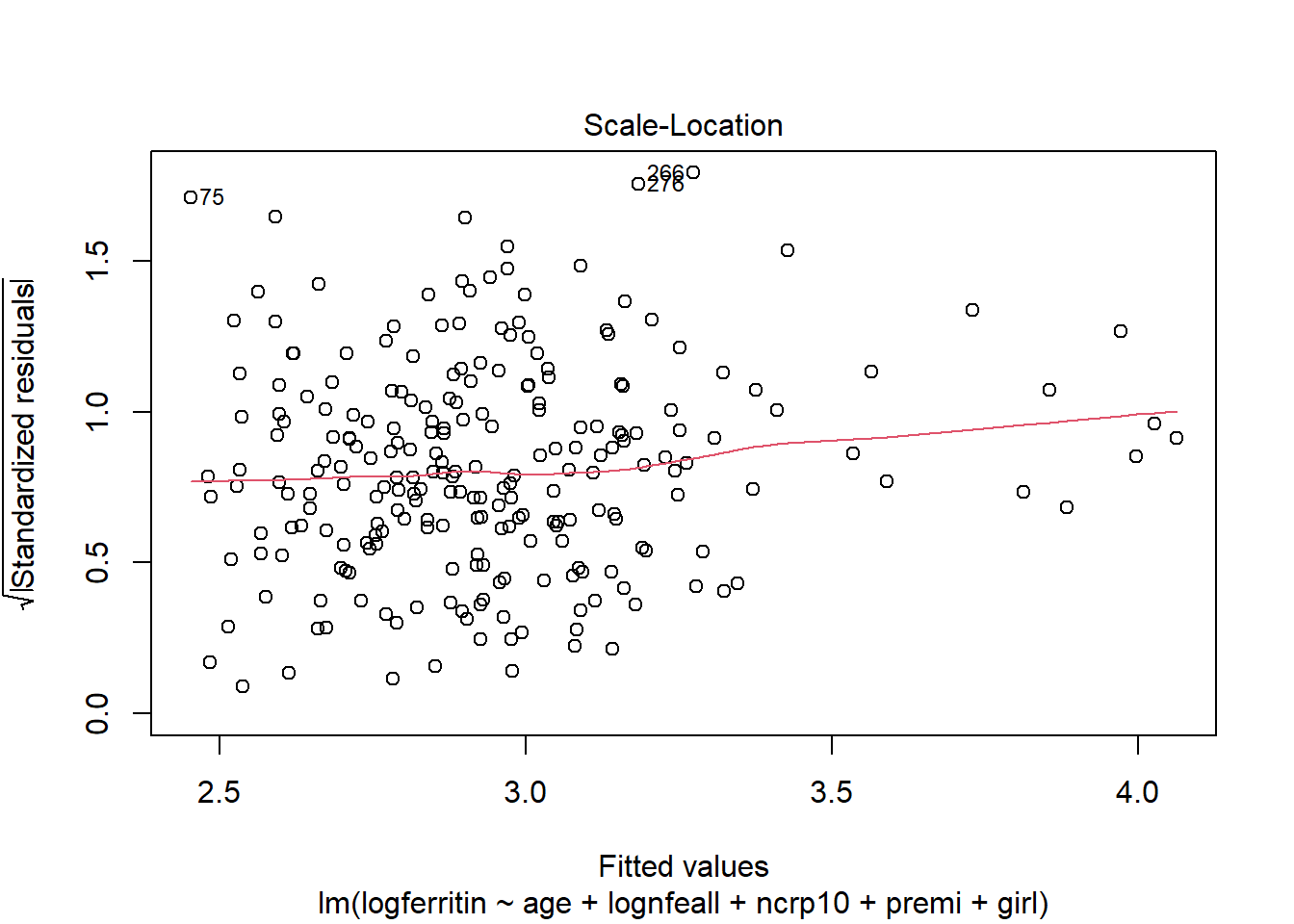
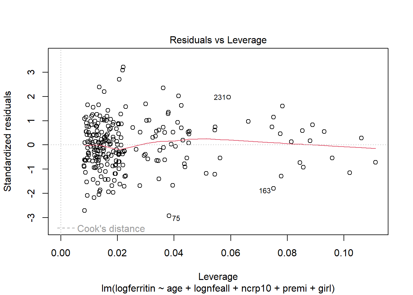
The predictor variables age, log dietary iron, and elevated C-reactive protein indicator have a significant relationship with log ferritin levels. When age increases by one month (with all other predictors held constant), log ferritin levels decrease by 0.0305. When log dietary iron increases by one unit log ferritin levels increase by 0.1479. For a child with elevated C-reactive protein levels, log ferritin is predicted to be 0.7941 higher compared to a child without. Being premature has a borderline significant negative effect on log ferritin, while being female has a borderline significant positive effect.

There are no issues with plot of residuals against fitted values - the variance appears to be constant and random.

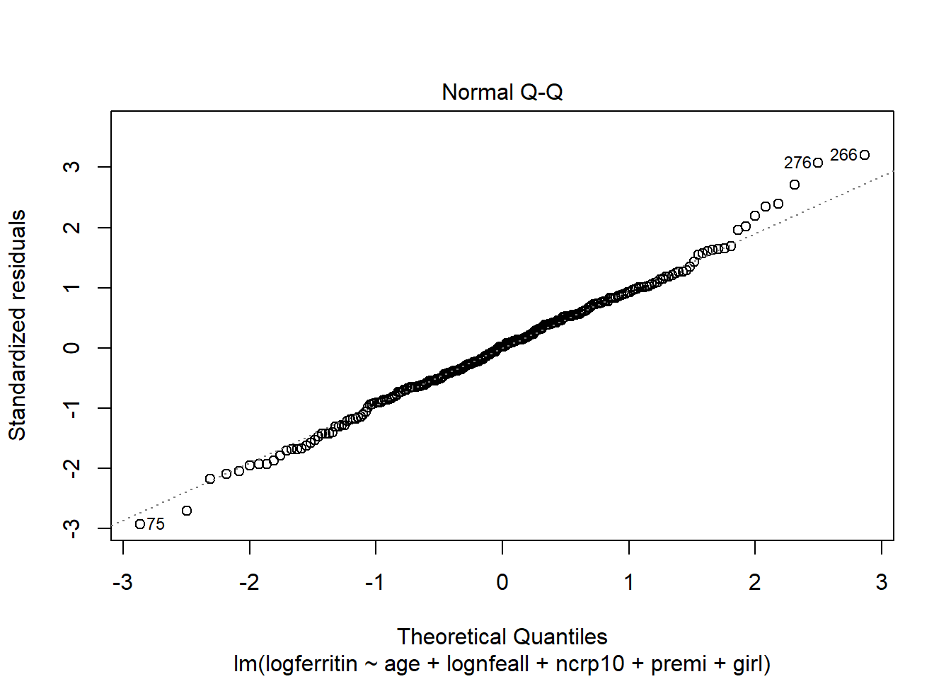
The normal qq plot indicates no cause for concern as the standardised residuals closely follow the standard normal quantiles.

There are a few outliers with square root standardised residuals around 1.75 (corresponding to 3 when squared).

The fourth plot indicates a couple of highly influential points - observations 75, 163 and 231. The influence of point 75 is due to a large standardised residual value (it is an outlier). This may be due to a measurement or transcription error, the ferritin value is 2.00 which is the lowest in the data set. It is also possible that there is additional natural variation that has not been accounted for by our model. Observations 163 and 231 have quite large residual values and this combined with their relatively high leverage makes them influential.