13 Rotavirus Burden
We have a survey open right now that we invite you to fill out.
This lesson follows a study for the World Health Organisation investigating the estimation of global burden of disease attributable to rotavirus. That is, counting the number of deaths globally due to rotavirus. The original research is presented by Julie Legler (St Olaf College).
The data discussed in the video was retrieved from the World Health Organisation (WHO) in 2004, and due to its estimated nature there have been some revisions between now and then. There has also been widespread implementation of the rotavirus vaccine that Julie discusses, so it is interesting and relevant for us to consider some more current data. Data for the year 2016 is the most recently available at the time of writing and provided for download on this page. Estimated proportions of diarrhoea deaths attributable to rotavirus were retrieved from Troeger et al. (2018), and all other data was sourced from the WHO website. The reported statistics will not align with the video, rather we can focus on comparing them to see how the vaccine has impacted the number of rotavirus deaths. The methodology used to obtain these values is directly translatable from the video.
Data
There is 1 file associated with this presentation. It contains the 2016 data you will need to complete the lesson tasks.
Video
Objectives
Tasks
0. Read and Format data
0a. Read in the data
First check you have installed the package readxl (see Section 2.6) and set the working directory (see Section 2.1), using instructions in Getting started with R.
Load the data into R.
The code has been hidden initially, so you can try to load the data yourself first before checking the solutions.
Code
#loads readxl package
library(readxl)

#loads the data file and names it rotavirus
rotavirus<-read_xlsx("Rotavirus Data.xlsx")

#view beginning of data frame
head(rotavirus)
Code
#loads readxl package
library(readxl)
Warning: package 'readxl' was built under R version 4.2.2Code
#loads the data file and names it rotavirus
rotavirus<-read_xlsx("Rotavirus Data.xlsx")

#view beginning of data frame
head(rotavirus)
# A tibble: 6 × 13
`WHO Region` World…¹ Count…² Country Under…³ Under…⁴ Diarr…⁵ TotFe…⁶ Femal…⁷
<chr> <chr> <chr> <chr> <dbl> <dbl> <dbl> <dbl> <dbl>
1 Eastern Medit… Low in… AFG Afghan… 5529. 79812 5.84e3 4.8 62.4
2 Europe Upper … ALB Albania 177. 331 2.58e0 1.66 79.7
3 Africa Lower … DZA Algeria 4741. 25016 1.01e3 3.05 77.5
4 Africa Lower … AGO Angola 5319. 98196 1.28e4 5.69 64.5
5 Americas High i… ATG Antigu… 7.36 11 0 2.00 77.8
6 Americas Upper … ARG Argent… 3740. 8219 8.02e1 2.29 79.3
# … with 4 more variables: TotHealthExpend <dbl>, InfantMortality <dbl>,
# EstimatedRotavirusProp <dbl>, ImmunisationPerc <dbl>, and abbreviated
# variable names ¹`World Bank Income Group`, ²`Country ISO Code`, ³Under5Pop,
# ⁴Under5Deaths, ⁵DiarrhoeaDeaths, ⁶TotFertility, ⁷FemaleLifeExpect
# ℹ Use `colnames()` to see all variable namesThis data frame contains information for 183 countries (Country), including their WHO Region, World Bank Income Group, and Country ISO Code. For each country in the year 2016 this includes the population under 5 years in thousands (Under5Pop), the number of deaths under 5 years (Under5Deaths), the number of deaths attributed to diarrhoea (DiarrhoeaDeaths), the total fertility rate (TotFertility), the life expectancy at birth for females (FemaleLifeExpect), the total health expenditure as a percentage of GDP (TotHealthExpend), the infant mortality rate per 1000 live births (InfantMortality), and the percentage of 1-year olds who had received a completed rotavirus vaccine dose in 2014 (ImmunisationPerc). The proportion of diarrhoea deaths due to rotavirus are given for 105 countries (EstimatedRotavirusProp).
1. Confidence Interval (mean proportion), Missing Data (overall mean)
1a. Confidence Interval (mean proportion)
Obtain the overall mean proportion of diarrhoea deaths due to rotavirus (EstimatedRotaVirusProp) and the corresponding 95% confidence interval.
How does our estimate for the mean proportion of diarrhoea deaths due to rotavirus (2016) compare to the mean proportion (2004) discussed in the video?
We calculate a confidence interval for the mean by using t.test() for a single set of data.
Code
t.test(rotavirus$EstimatedRotavirusProp) Code
t.test(rotavirus$EstimatedRotavirusProp)
    One Sample t-test

data:  rotavirus$EstimatedRotavirusProp
t = 11.711, df = 104, p-value < 2.2e-16
alternative hypothesis: true mean is not equal to 0
95 percent confidence interval:
 0.1999397 0.2814555
sample estimates:
mean of x
0.2406976
We can say with 95% confidence that the true mean proportion of diarrhoea deaths due to rotavirus in 2016 was between 0.1999 and 0.2815, with a best estimate of 0.2407. This is less than the mean proportion of 0.36 recorded in 2004.
1b. Replace Missing Data (overall mean)
Use the mean proportion as an estimate for missing EstimatedRotaVirusProp values.
Create a new variable ConstantRotavirusProp containing existing EstimatedRotavirusProp values, and replace the missing proportions with the mean proportion estimate.
To calculate the total estimated rotavirus deaths in 2016, multiply the number of DiarrhoeaDeaths by the proportion attributed to rotavirus for each country (where missing data is the estimated by the mean proportion). sum() these to find the total.
Code
#new variable, pre-fill with available rotavirus proportions
rotavirus$ConstantRotavirusProp<-rotavirus$EstimatedRotavirusProp

#assign missing entries of this variable to be equal to the mean rotavirus proportion
rotavirus$ConstantRotavirusProp[which(is.na(rotavirus$ConstantRotavirusProp))]<-0.2407
Code
#total estimated deaths
sum(rotavirus$DiarrhoeaDeaths*rotavirus$ConstantRotavirusProp)
Code
#new variable, pre-fill with available rotavirus proportions
rotavirus$ConstantRotavirusProp<-rotavirus$EstimatedRotavirusProp

#assign missing entries of this variable to be equal to the mean rotavirus proportion
rotavirus$ConstantRotavirusProp[which(is.na(rotavirus$ConstantRotavirusProp))]<-0.2407
Code
#total estimated deaths
sum(rotavirus$DiarrhoeaDeaths*rotavirus$ConstantRotavirusProp)
[1] 119376.82. Bootstrap Confidence Interval, Histogram (sum of rotavirus deaths)
2a. Bootstrap Confidence Interval
Construct a bootstrap confidence interval for the sum of diarrhoea deaths attributable to rotavirus, continuing to use the mean rotavirus proportion as an estimate for countries where data is missing (ConstantRotavirusProp).
Perform bootstrap for the sum.
Code
library(boot)

#set seed so you get the same results when running again
set.seed(402)

#function that calculates the sum from the bootstrapped samples
sumFun<-function(data,indices){
  dataInd<-data[indices,]
  sumdata<-sum(dataInd$DiarrhoeaDeaths*dataInd$ConstantRotavirusProp)
  return(sumdata)
}

#bootstrap sum of diarrhoea deaths attributable to rotavirus.
#create object called sumBoot with the output of the bootstrapping procedure
sumBoot<-boot(rotavirus,statistic=sumFun, R=10000)
Use boot.ci() to calculate a percentile confidence interval.
Code
#percentile (type="perc") confidence interval
percCi<-boot.ci(sumBoot,type="perc")

#check lower and upper limits from percentile interval object
percCi$percent[4:5]
Code
library(boot)Warning: package 'boot' was built under R version 4.2.2Code
#set seed so you get the same results when running again
set.seed(402)

#function that calculates the sum from the bootstrapped samples
sumFun<-function(data,indices){
  dataInd<-data[indices,]
  sumdata<-sum(dataInd$DiarrhoeaDeaths*dataInd$ConstantRotavirusProp)
  return(sumdata)
}

#bootstrap sum of diarrhoea deaths attributable to rotavirus.
#create object called sumBoot with the output of the bootstrapping procedure
sumBoot<-boot(rotavirus,statistic=sumFun, R=10000)
Code
#percentile (type="perc") confidence interval
percCi<-boot.ci(sumBoot,type="perc")

#check lower and upper limits from percentile interval object
percCi$percent[4:5]
[1] 51464.73 236036.512b. Histogram
Create a graph showing the distribution of the sum of the bootstrap samples with a density curve and 95% confidence interval limits plotted on top.
How does this bootstrap confidence interval for the number of rotavirus deaths compare to the bootstrap confidence interval for the number of rotavirus deaths discussed in the video?
What factors could have contributed to this change?
Code
#plot density histogram of bootstrap results
hist(sumBoot$t,breaks=20,freq=F, xlab="Total Rotavirus Deaths",
    main="Sum of Rotavirus Deaths in 2016")

#add a smoothed line to show the distribution
lines(density(sumBoot$t),col="skyblue3",lwd=2)

#95% ci limits
abline(v=percCi$percent[4:5],col="skyblue2",lty=2)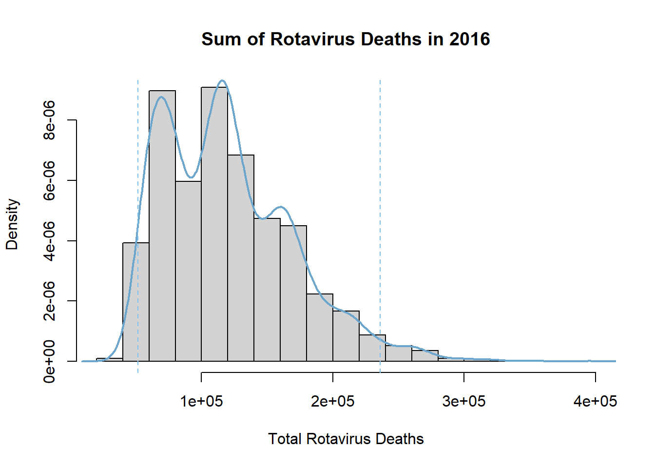
The bootstrapped sums follow a right-skewed distribution with mean of 119376.8. This mean of sums matches the estimated sum of diarrhoea deaths attributable to rotavirus we calculated earlier, and the distribution of bootstrapped sum estimates around it give an indication of the amount of variability in our estimate due to sampling. This 95% percentile interval is from 51,464.73 to 236,036.51, which is a very large range.
The corresponding bootstrap confidence interval in the video is from 362,363.04 to 1,157,640.34. This interval encompasses much greater sums of rotavirus deaths and is entirely above our interval for 2016. The reduction in estimated rotavirus deaths may be due to improved awareness, better sanitation, nutrition and healthcare, and the implementation of the rotavirus vaccine.
3. Missing Data (stratification)
3a. Stratification by Female Life Expectancy
Use female life expectancy (FemaleLifeExpect) to define the five strata.
Code
#define object with FemaleLifeExpect values in decreasing order
rotavirusFLE<-rotavirus$FemaleLifeExpect[order(-rotavirus$FemaleLifeExpect)]
Code
#calculate difference between consecutive female life expectancies
diff<-rotavirusFLE[1:182]-rotavirusFLE[2:183]

#establish cut-off between strata

#difference vector entry number
which(diff>0.60)
#actual difference in life expectancy
diff[which(diff>0.60)]
Ignoring differences 178, 179, 180, 181 and 182 as change points due to their lack of separation leaves four change points to define five strata.
Confirm this decision by visualising the ordered FemaleLifeExpect with change points indicated.
Code
#x axis is index from 1 to 183, y axis is female life expectancy.
#type="o" plots points joined with lines
plot(1:length(rotavirusFLE),rotavirusFLE,type="o",col="orange",
 pch=20,ylab="Female Life Expectancy (years)", xlab="Country Index")

#add lines at proposed change points between strata
abline(v=c(31,103,142,175),col="skyblue2",lty=2)
If you open this plot in a new window (button in the top right of the plot), you should see the proposed change points line up with the biggest drops female life expectancy. This provides a justification for grouping according to these categories.
Extract the FemaleLifeExpect ages corresponding to these cut-offs, and define a new variable StrataFemaleLifeExpect that groups FemaleLifeExpect into categories.
Code
#subset entries corresponding to cut-offs
rotavirusFLE[c(31,103,142,175)]
Code
#initially define new variable as all 0s, same number of rows as data frame
rotavirus$StrataFemaleLifeExpect<-rep(0,nrow(rotavirus))

#life expectancy greater than or equal to 82.34 in first strata (1)
rotavirus$StrataFemaleLifeExpect[which(rotavirus$FemaleLifeExpect>=82.34)]<-1

#life expectancy greater than or equal to 74.78 and less than 82.34 in second strata (2)
rotavirus$StrataFemaleLifeExpect[which(rotavirus$FemaleLifeExpect>=74.78&rotavirus$FemaleLifeExpect<82.34)]<-2

#life expectancy greater than or equal to 67.26 and less than 74.78 in third strata (3)
rotavirus$StrataFemaleLifeExpect[which(rotavirus$FemaleLifeExpect>=67.26&rotavirus$FemaleLifeExpect<74.78)]<-3

#life expectancy greater than or equal to 60.81 and less than 67.26 in fourth strata (4)
rotavirus$StrataFemaleLifeExpect[which(rotavirus$FemaleLifeExpect>=60.81&rotavirus$FemaleLifeExpect<67.26)]<-4

#life expectancy less than 60.81 in fifth strata (5)
rotavirus$StrataFemaleLifeExpect[which(rotavirus$FemaleLifeExpect<60.81)]<-5
Code
#define object with FemaleLifeExpect values in decreasing order
rotavirusFLE<-rotavirus$FemaleLifeExpect[order(-rotavirus$FemaleLifeExpect)]
Code
#calculate difference between consecutive female life expectancies
diff<-rotavirusFLE[1:182]-rotavirusFLE[2:183]

#establish cut-off between strata

#difference vector entry number
which(diff>0.60)
[1] 1 31 103 142 175 178 179 180 181 182Code
#actual difference in life expectancy
diff[which(diff>0.60)]
[1] 1.29 0.63 0.69 0.64 0.74 0.74 0.78 0.62 4.28 2.45Ignoring differences 178, 179, 180, 181 and 182 as change points due to their lack of separation leaves four change points to define five strata.
Confirm this decision by visualising the ordered FemaleLifeExpect with change points indicated.
Code
#x axis is index from 1 to 183, y axis is female life expectancy.
#type="o" plots points joined with lines
plot(1:length(rotavirusFLE),rotavirusFLE,type="o",col="orange",
 pch=20,ylab="Female Life Expectancy (years)", xlab="Country Index")

#add lines at proposed change points between strata
abline(v=c(31,103,142,175),col="skyblue2",lty=2)
If you open this plot in a new window (button in the top right of the plot), you should see the proposed change points line up with the biggest drops female life expectancy. This provides a justification for grouping according to these categories.
Extract the FemaleLifeExpect ages corresponding to these cut-offs, and define a new variable StrataFemaleLifeExpect that groups FemaleLifeExpect into categories.
Code
#subset entries corresponding to cut-offs
rotavirusFLE[c(31,103,142,175)]
[1] 82.34 74.78 67.26 60.81Code
#initially define new variable as all 0s, same number of rows as data frame
rotavirus$StrataFemaleLifeExpect<-rep(0,nrow(rotavirus))

#life expectancy greater than or equal to 82.34 in first strata (1)
rotavirus$StrataFemaleLifeExpect[which(rotavirus$FemaleLifeExpect>=82.34)]<-1

#life expectancy greater than or equal to 74.78 and less than 82.34 in second strata (2)
rotavirus$StrataFemaleLifeExpect[which(rotavirus$FemaleLifeExpect>=74.78&
                                             rotavirus$FemaleLifeExpect<82.34)]<-2

#life expectancy greater than or equal to 67.26 and less than 74.78 in third strata (3)
rotavirus$StrataFemaleLifeExpect[which(rotavirus$FemaleLifeExpect>=67.26&
                                             rotavirus$FemaleLifeExpect<74.78)]<-3

#life expectancy greater than or equal to 60.81 and less than 67.26 in fourth strata (4)
rotavirus$StrataFemaleLifeExpect[which(rotavirus$FemaleLifeExpect>=60.81&
                                            rotavirus$FemaleLifeExpect<67.26)]<-4

#life expectancy less than 60.81 in fifth strata (5)
rotavirus$StrataFemaleLifeExpect[which(rotavirus$FemaleLifeExpect<60.81)]<-5
3b. Strata Mean for Missing Data
Calculate the proportion average of EstimatedRotavirusProp in each stratum using tapply().
Then calculate the sum of rotavirus deaths overall using these values for the missing data.
Use the mean strata proportion as an estimate for missing EstimatedRotaVirusProp values.
Code
tapply(rotavirus$EstimatedRotavirusProp,INDEX=rotavirus$StrataFemaleLifeExpect,FUN=mean,na.rm=T)Create a new variable FLERotavirusProp containing existing EstimatedRotavirusProp values, and replace the missing proportions with the relevant mean proportion estimate.
Code
#new variable, pre-fill with available rotavirus proportions
rotavirus$FLERotavirusProp<-rotavirus$EstimatedRotavirusProp

#assign missing entries of this variable that correspond to a value of 1 in the strata variable,
#equal to the mean proportion for that strata
rotavirus$FLERotavirusProp[which(is.na(rotavirus$EstimatedRotavirusProp)&
                (rotavirus$StrataFemaleLifeExpect==1))]<-0.2144838

#assign missing entries of this variable that correspond to a value of 2 in the strata variable,
#equal to the mean proportion for that strata
rotavirus$FLERotavirusProp[which(is.na(rotavirus$EstimatedRotavirusProp)&
                (rotavirus$StrataFemaleLifeExpect==2))]<-0.2592195

#assign missing entries of this variable that correspond to a value of 3 in the strata variable,
#equal to the mean proportion for that strata
rotavirus$FLERotavirusProp[which(is.na(rotavirus$EstimatedRotavirusProp)&
                (rotavirus$StrataFemaleLifeExpect==3))]<-0.2236106

#assign missing entries of this variable that correspond to a value of 4 in the strata variable,
#equal to the mean proportion for that strata
rotavirus$FLERotavirusProp[which(is.na(rotavirus$EstimatedRotavirusProp)&
                (rotavirus$StrataFemaleLifeExpect==4))]<-0.2474089


#assign missing entries of this variable that correspond to a value of 5 in the strata variable,
#equal to the mean proportion for that strata
rotavirus$FLERotavirusProp[which(is.na(rotavirus$EstimatedRotavirusProp)&
                (rotavirus$StrataFemaleLifeExpect==5))]<-0.1972870
Calculate the sum of rotavirus deaths as before, using the FLERotavirusProp values where missing data is estimated using female life expectancy strata means.
Code
sum(rotavirus$DiarrhoeaDeaths*rotavirus$FLERotavirusProp)Use the mean strata proportion as an estimate for missing EstimatedRotaVirusProp values.
Code
tapply(rotavirus$EstimatedRotavirusProp,INDEX=rotavirus$StrataFemaleLifeExpect,FUN=mean,na.rm=T) 1 2 3 4 5
0.2144838 0.2592195 0.2236106 0.2474089 0.1972870 Create a new variable FLERotavirusProp containing existing EstimatedRotavirusProp values, and replace the missing proportions with the relevant mean proportion estimate.
Code
#new variable, pre-fill with available rotavirus proportions
rotavirus$FLERotavirusProp<-rotavirus$EstimatedRotavirusProp

#assign missing entries of this variable that correspond to a value of 1 in the strata variable,
#equal to the mean proportion for that strata
rotavirus$FLERotavirusProp[which(is.na(rotavirus$EstimatedRotavirusProp)&
                (rotavirus$StrataFemaleLifeExpect==1))]<-0.2144838

#assign missing entries of this variable that correspond to a value of 2 in the strata variable,
#equal to the mean proportion for that strata
rotavirus$FLERotavirusProp[which(is.na(rotavirus$EstimatedRotavirusProp)&
                (rotavirus$StrataFemaleLifeExpect==2))]<-0.2592195

#assign missing entries of this variable that correspond to a value of 3 in the strata variable,
#equal to the mean proportion for that strata
rotavirus$FLERotavirusProp[which(is.na(rotavirus$EstimatedRotavirusProp)&
                (rotavirus$StrataFemaleLifeExpect==3))]<-0.2236106

#assign missing entries of this variable that correspond to a value of 4 in the strata variable,
#equal to the mean proportion for that strata
rotavirus$FLERotavirusProp[which(is.na(rotavirus$EstimatedRotavirusProp)&
                (rotavirus$StrataFemaleLifeExpect==4))]<-0.2474089


#assign missing entries of this variable that correspond to a value of 5 in the strata variable,
#equal to the mean proportion for that strata
rotavirus$FLERotavirusProp[which(is.na(rotavirus$EstimatedRotavirusProp)&
                (rotavirus$StrataFemaleLifeExpect==5))]<-0.1972870
Calculate the sum of rotavirus deaths as before, using the FLERotavirusProp values where missing data is estimated using female life expectancy strata means.
Code
sum(rotavirus$DiarrhoeaDeaths*rotavirus$FLERotavirusProp)[1] 118973.9Use total health expenditure as a percentage of GDP (TotHealthExpend) to define the five strata.
Compare the estimates of rotavirus deaths using FemaleLifeExpect and TotHealthExpend to fill in missing values with the estimate gained using an overall average proportion for missing values.
4. Scatter Plots, Correlations (predictors and response)
4a. Fertility, Female Life Expectancy, Health Expenditure, Infant Mortality
Investigate individually the four predictors (TotFertility, FemaleLifeExpect, TotHealthExpend and InfantMortality).
Examine scatter plots and the correlation coefficients between these predictors and the known proportions (EstimatedRotavirusDeaths) for the 105 countries.
Describe the relationship between each of these predictors and EstimatedRotavirusProp. Is this what you would expect, and if not, what could explain it?
Code
#create new data frame where rows with missing estimated rotavirus proportions are removed
rotavirusFull<-rotavirus[!is.na(rotavirus$EstimatedRotavirusProp),]

#scatter plot
plot(rotavirusFull$FemaleLifeExpect,rotavirusFull$EstimatedRotavirusProp,xlab="Female Life Expectancy (years)",pch=15,col="purple",ylab="Estimated Diarrhoea Deaths due to Rotavirus (proportion)")

#correlation between values
cor(rotavirusFull$FemaleLifeExpect,rotavirusFull$EstimatedRotavirusProp)
Repeat these analyses for TotFertility, TotHealthExpend and InfantMortality. Make sure to remove any rows containing missing data for these variables, otherwise the corr() function will return NA.
Code
#create new data frame where rows with missing estimated rotavirus proportions are removed
rotavirusFull<-rotavirus[!is.na(rotavirus$EstimatedRotavirusProp),]

#scatter plot
plot(rotavirusFull$FemaleLifeExpect,rotavirusFull$EstimatedRotavirusProp,xlab="Female Life Expectancy (years)",pch=15,col="purple",ylab="Estimated Diarrhoea Deaths due to Rotavirus (proportion)")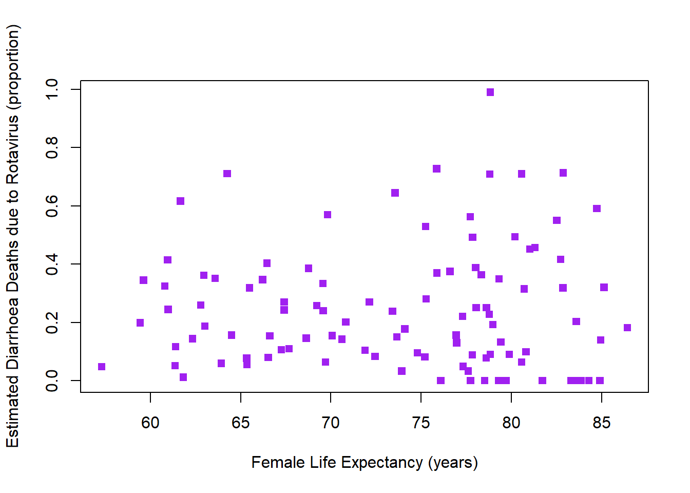
Code
#correlation between values
cor(rotavirusFull$FemaleLifeExpect,rotavirusFull$EstimatedRotavirusProp)
[1] -0.001615984Very slight negative relationship, as female life expectancy increases the estimated proportion of diarrhoea deaths from rotavirus decrease. This is unlikely to be significant however.
Code
plot(rotavirusFull$TotFertility,rotavirusFull$EstimatedRotavirusProp,xlab="Total Fertility Rate",pch=15,col="pink",ylab="Estimated Diarrhoea Deaths due to Rotavirus (proportion)")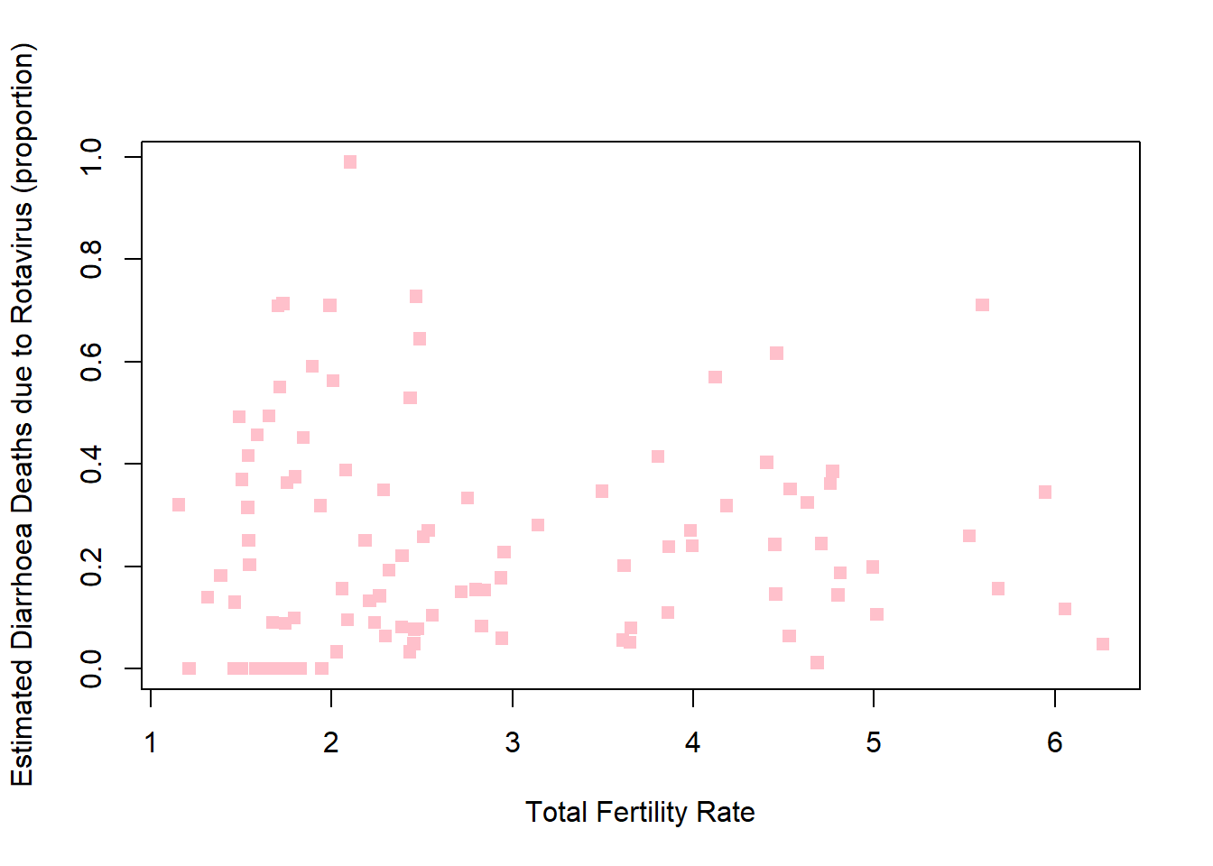
Code
cor(rotavirusFull$TotFertility,rotavirusFull$EstimatedRotavirusProp)[1] 0.03986769Slight positive relationship, as total fertility increases the estimated proportion of diarrhoea deaths from rotavirus increase.
Code
rotavirusFull2<-rotavirusFull[!is.na(rotavirusFull$TotHealthExpend),]

plot(rotavirusFull2$TotHealthExpend,rotavirusFull2$EstimatedRotavirusProp,xlab="Total Health Expenditure (% GDP)",pch=15,col="blue",ylab="Estimated Diarrhoea Deaths due to Rotavirus (proportion)")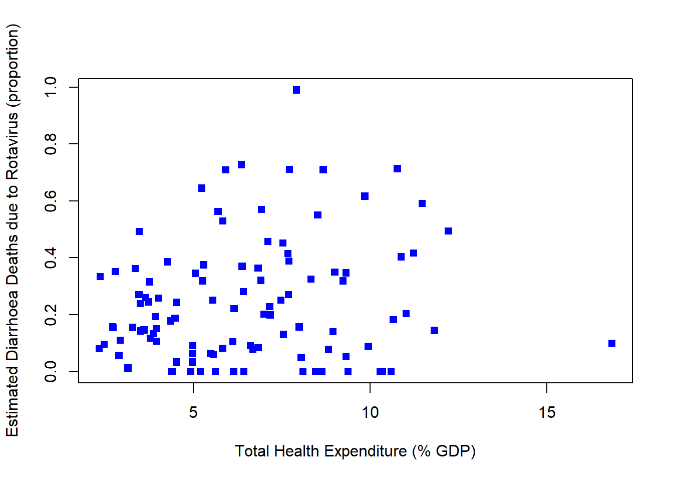
Code
cor(rotavirusFull2$TotHealthExpend,rotavirusFull2$EstimatedRotavirusProp)[1] 0.1527748Positive relationship, as total health expenditure increases the estimated proportion of diarrhoea deaths from rotavirus increase.
Code
plot(rotavirusFull$InfantMortality,rotavirusFull$EstimatedRotavirusProp,xlab="Infant Mortality (per 1000 live births)",pch=15,col="red", ylab="Estimated Diarrhoea Deaths due to Rotavirus (proportion)")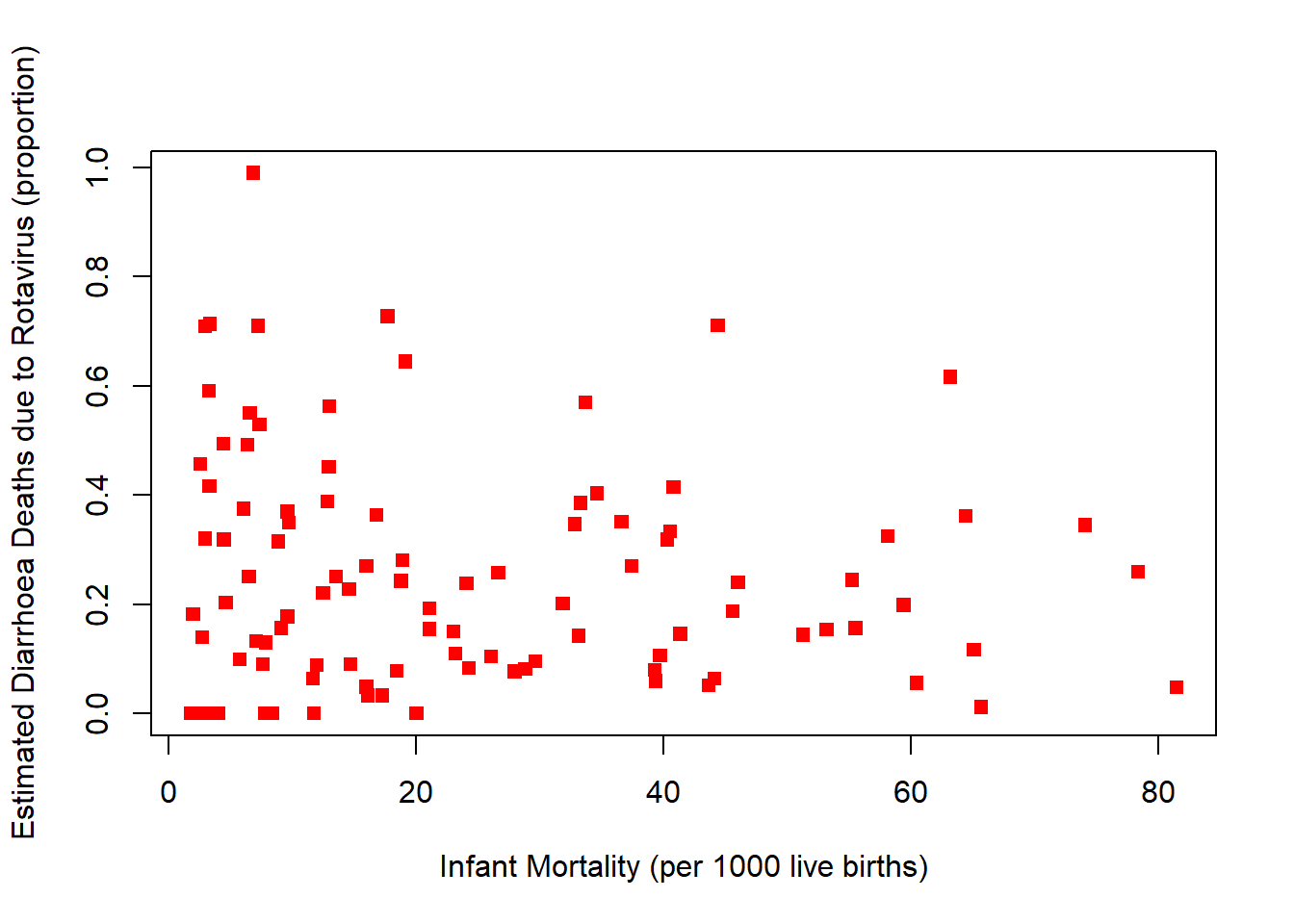
Code
cor(rotavirusFull$InfantMortality,rotavirusFull$EstimatedRotavirusProp)[1] -0.04307308Slight negative relationship, as infant mortality increases the estimated proportion of diarrhoea deaths from rotavirus decrease.
4b Immunisation Rates.
Examine the relationship between rotavirus vaccination rates (ImmunisationPerc) and the estimated proportion of rotavirus deaths (EstimatedRotavirusProp).
What kind of relationship can you see? Is it what you would expect, if not, why might we be observing this relationship?
Code
#remove rows where immunisation percentage is missing
rotavirusFull3<-rotavirusFull[!is.na(rotavirusFull$ImmunisationPerc),]

#scatter plot
plot(rotavirusFull3$ImmunisationPerc,rotavirusFull3$EstimatedRotavirusProp,xlab="Rotavirus Immunisation (% at 1 year old)",pch=15,col="green", ylab="Estimated Diarrhoea Deaths due to Rotavirus (proportion)")

#correlation between variables
cor(rotavirusFull3$ImmunisationPerc,rotavirusFull3$EstimatedRotavirusProp)
Code
#remove rows where immunisation percentage is missing
rotavirusFull3<-rotavirusFull[!is.na(rotavirusFull$ImmunisationPerc),]

#scatter plot
plot(rotavirusFull3$ImmunisationPerc,rotavirusFull3$EstimatedRotavirusProp,xlab="Rotavirus Immunisation (% at 1 year old)",pch=15,col="green", ylab="Estimated Diarrhoea Deaths due to Rotavirus (proportion)")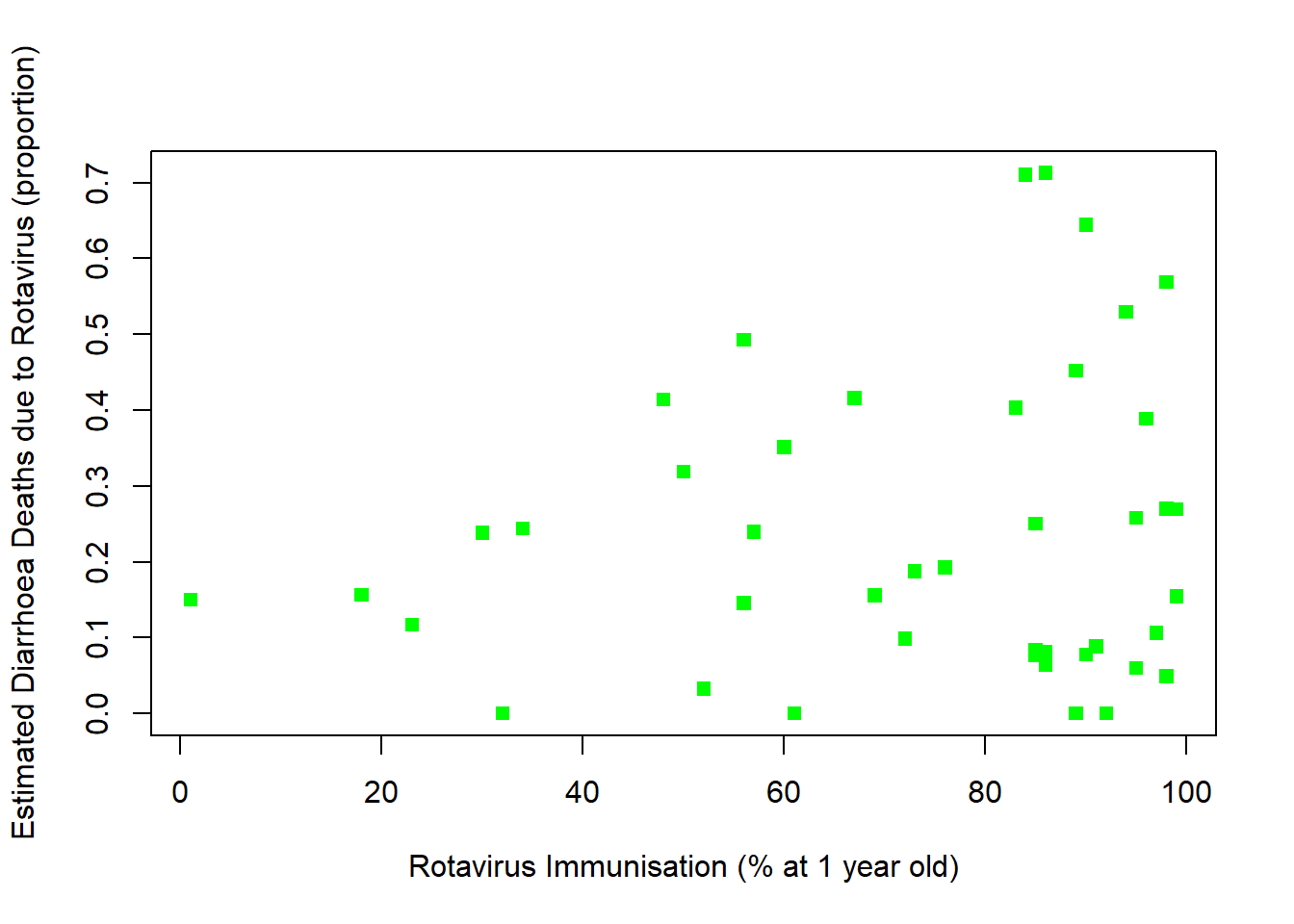
Code
#correlation between variables
cor(rotavirusFull3$ImmunisationPerc,rotavirusFull3$EstimatedRotavirusProp)
[1] 0.1295355There is a positive relationship, as immunisation percentage goes up so does the estimated proportion of diarrhoea deaths due to rotavirus.
This seems counter-intuitive as we would expect the proportion of diarrhoea deaths due to rotavirus to decrease with increasing immunisation coverage. Some reasons we do not see a negative relationship between immunisation rates and proportion of diarrhoea deaths attributable to rotavirus are:
Limited data
The greatest amount of data is available for countries which have high immunisation rates, there are very few observations where immunisation rates are less than 40% and the relationship may be different here.
The immunisation statistics are for 1 year olds in 2014. Children older than 2 years in 2016 would have been due for these immunisations earlier and the coverage was lower then.
Countries with high proportions of diarrhoea deaths due to rotavirus virus were likely prioritised in the vaccine roll-out.
5. Missing Data (linear regression)
5a. Simple Linear Regression
Predict all the proportions using FemaleLifeExpect as a predictor in a simple regression. (105 countries have a proportion).
Compare the result from this procedure with the result obtained by using strata based on this variable in Task 3.
Use the function lm() to fit this model.
Code
#linear model
FLEMod<-lm(EstimatedRotavirusProp~FemaleLifeExpect,data=rotavirus)

#view fitted model
summary(FLEMod)
Once the model is fitted we can calculate the predicted values
Code
#use fitted model and values in rotavirus data frame to predict estimated rotavirus proportions
predFLE<-predict(FLEMod,newdata=rotavirus)
#total number of rotavirus deaths
sum(rotavirus$DiarrhoeaDeaths*predFLE,na.rm=T)
#residual checks
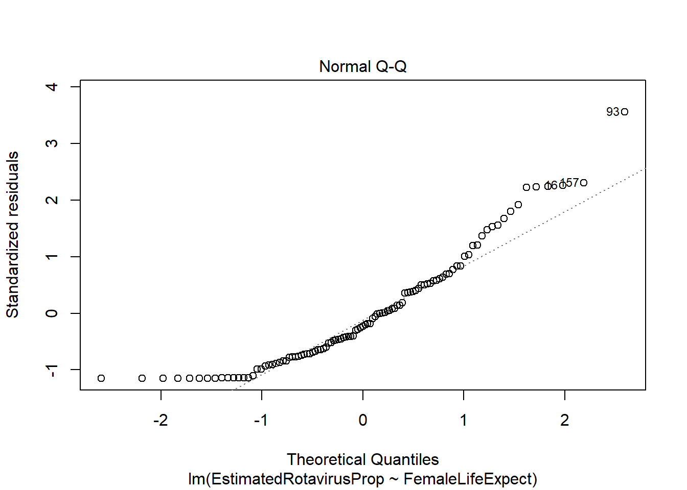
plot(FLEMod)Code
#linear model
FLEMod<-lm(EstimatedRotavirusProp~FemaleLifeExpect,data=rotavirus)

#view fitted model
summary(FLEMod)
Call:
lm(formula = EstimatedRotavirusProp ~ FemaleLifeExpect, data = rotavirus)

Residuals:
     Min       1Q   Median       3Q      Max
-0.24060 -0.16119 -0.04814  0.11020  0.74942

Coefficients:
                   Estimate Std. Error t value Pr(>|t|)
(Intercept)       2.440e-01  2.019e-01   1.208    0.230
FemaleLifeExpect -4.458e-05  2.718e-03  -0.016    0.987

Residual standard error: 0.2116 on 103 degrees of freedom
  (78 observations deleted due to missingness)
Multiple R-squared:  2.611e-06, Adjusted R-squared:  -0.009706
F-statistic: 0.000269 on 1 and 103 DF,  p-value: 0.9869
Code
#residual checks
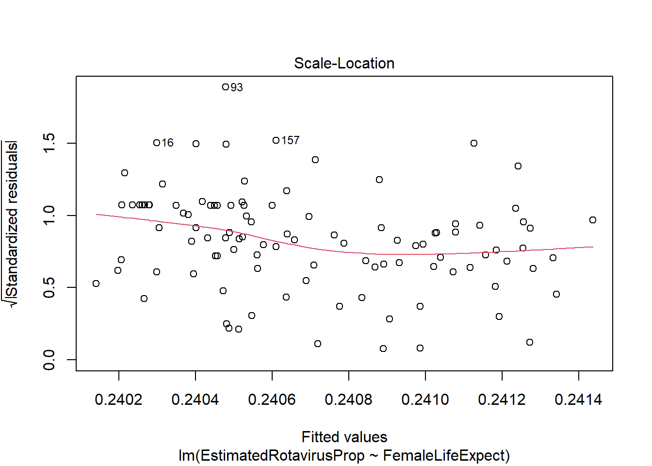
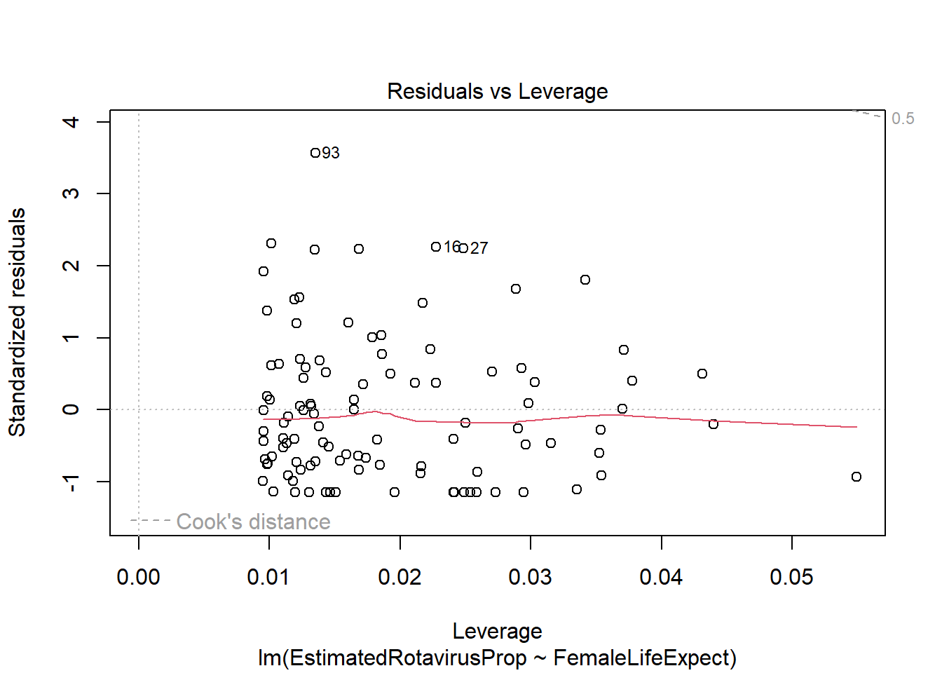
plot(FLEMod)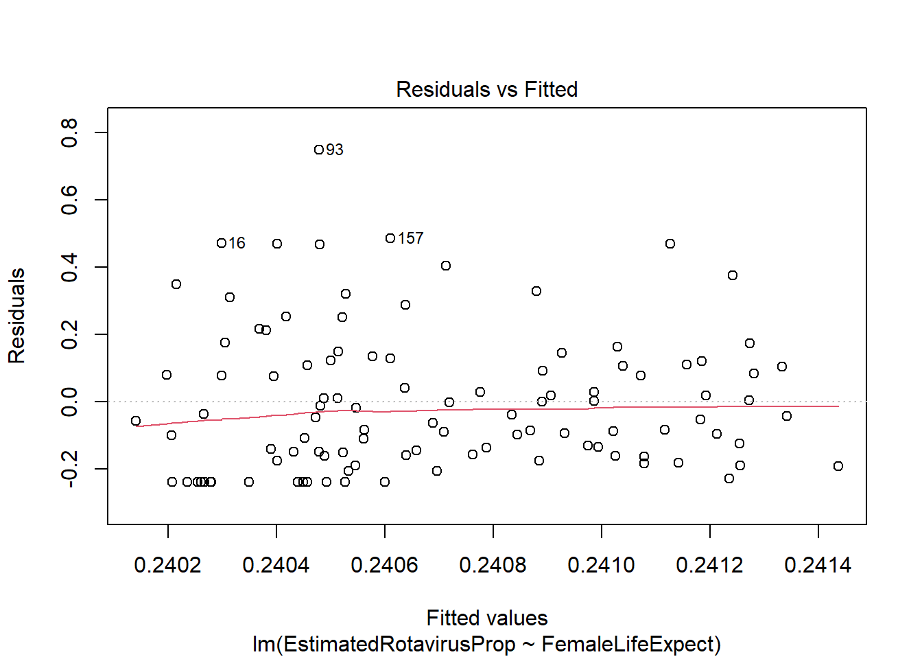
Code
#use fitted model and values in rotavirus data frame to predict estimated rotavirus proportions
predFLE<-predict(FLEMod,newdata=rotavirus)

#total number of rotavirus deaths
sum(rotavirus$DiarrhoeaDeaths*predFLE,na.rm=T)
[1] 138583.7Using female life expectancy as a continuous predictor in a linear regression results in a higher estimated sum of diarrhoea deaths attributable to rotavirus compared to using it categorically to define strata. 138,583.7 against 118,973.9.
However, there appear to be some problems with this fitted model. The residuals are not standard normally distributed - as shown by their departure from the quantiles on the QQ-plot and the increased number of large positive residuals relative to negative residuals.
5b. Multiple Linear Regression
Include the remaining predictors TotFertility, TotHealthExpend and InfantMortality in the regression, then using this model to predict the missing proportions.
How does this compare to other estimates of total rotavirus deaths in 2016?
Fit linear model.
Code
#linear model
ALLMod<-lm(EstimatedRotavirusProp~FemaleLifeExpect+TotFertility+TotHealthExpend+InfantMortality,data=rotavirus)
#view fitted model
summary(ALLMod)
#anova
anova(ALLMod)
#residuals
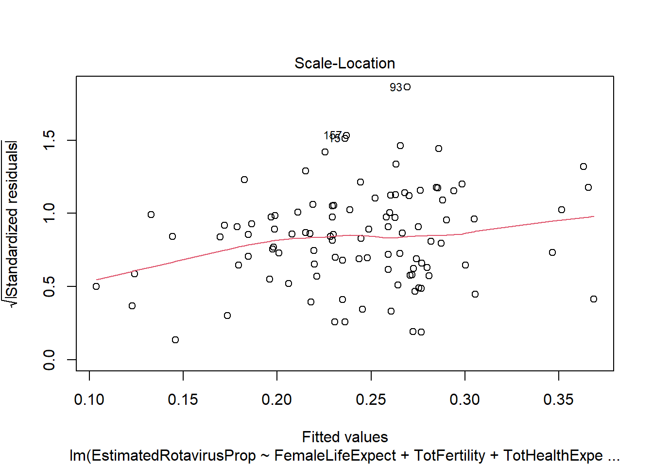
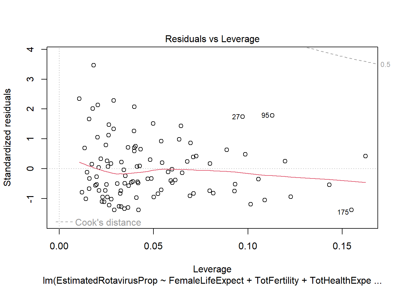
plot(ALLMod)Use results to calculated predicted values.
Code
#use fitted model and values in rotavirus data frame to predict estimated rotavirus proportions
predALL<-predict(ALLMod,newdata=rotavirus)

#total number of rotavirus deaths
sum(rotavirus$DiarrhoeaDeaths*predALL,na.rm=T)
Code
#linear model
ALLMod<-lm(EstimatedRotavirusProp~FemaleLifeExpect+TotFertility+TotHealthExpend+InfantMortality,data=rotavirus)

#view fitted model
summary(ALLMod)
Call:
lm(formula = EstimatedRotavirusProp ~ FemaleLifeExpect + TotFertility +
    TotHealthExpend + InfantMortality, data = rotavirus)

Residuals:
     Min       1Q   Median       3Q      Max
-0.28560 -0.15282 -0.05648  0.12420  0.72064

Coefficients:
                  Estimate Std. Error t value Pr(>|t|)
(Intercept)       0.333086   0.640359   0.520    0.604
FemaleLifeExpect -0.003262   0.007529  -0.433    0.666
TotFertility      0.055618   0.038076   1.461    0.147
TotHealthExpend   0.012985   0.008281   1.568    0.120
InfantMortality  -0.003872   0.002934  -1.320    0.190

Residual standard error: 0.2098 on 98 degrees of freedom
  (80 observations deleted due to missingness)
Multiple R-squared:  0.057, Adjusted R-squared:  0.01851
F-statistic: 1.481 on 4 and 98 DF,  p-value: 0.2138
Code
#anova
anova(ALLMod)
Analysis of Variance Table
Response: EstimatedRotavirusProp
Df Sum Sq Mean Sq F value Pr(>F)
FemaleLifeExpect 1 0.0021 0.002130 0.0484 0.82635
TotFertility 1 0.0458 0.045761 1.0393 0.31049
TotHealthExpend 1 0.1363 0.136252 3.0946 0.08167 .
InfantMortality 1 0.0767 0.076687 1.7417 0.18999
Residuals 98 4.3149 0.044029
---
Signif. codes: 0 '***' 0.001 '**' 0.01 '*' 0.05 '.' 0.1 ' ' 1Code
#residuals
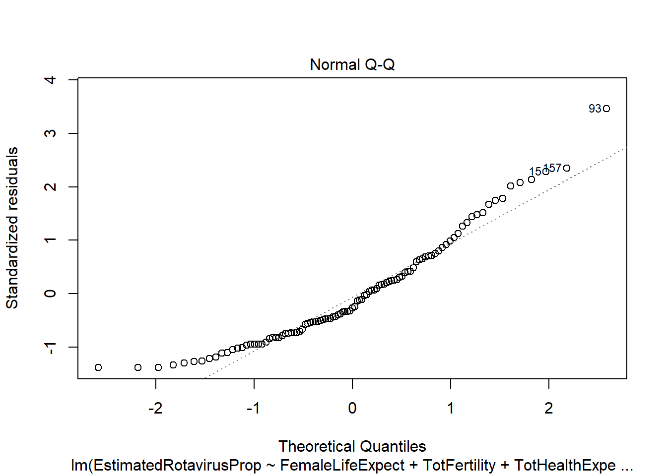
plot(ALLMod)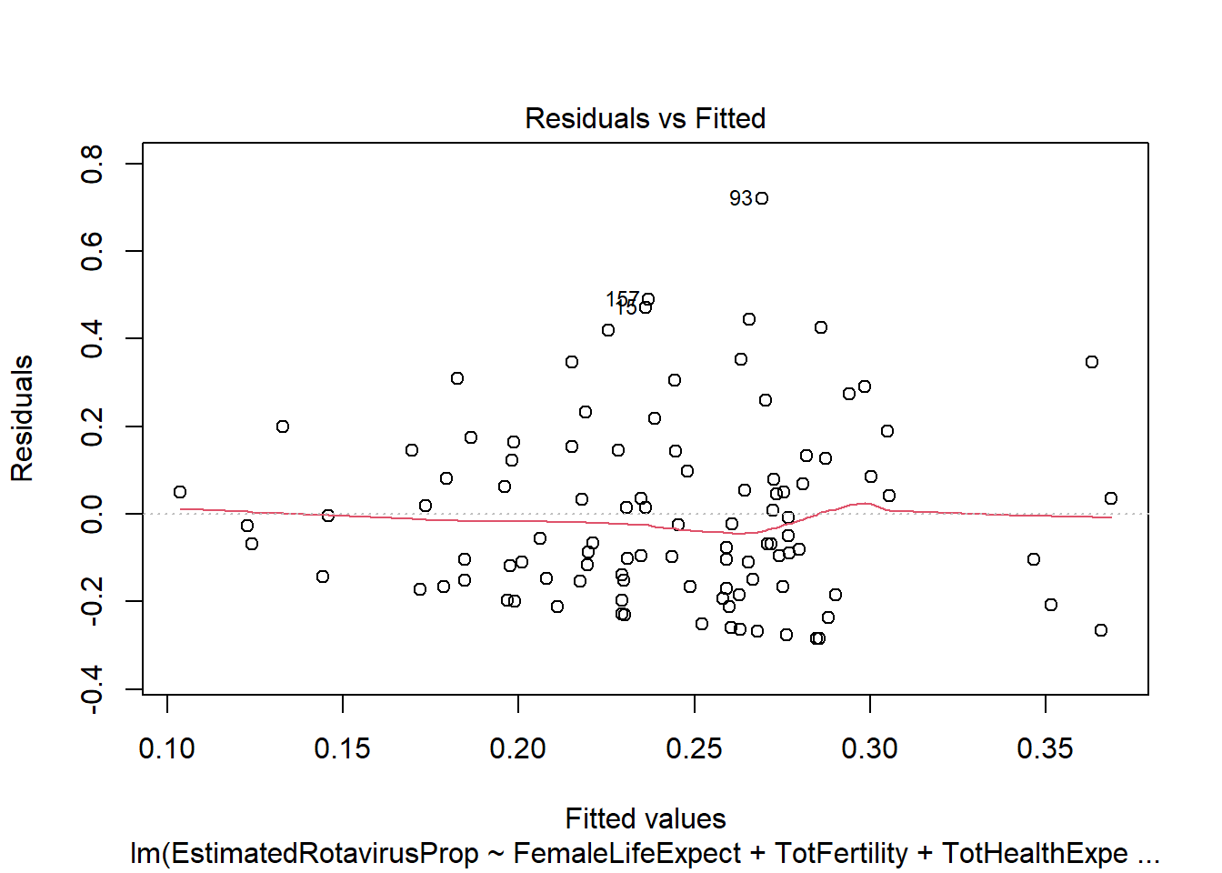
Code
#use fitted model and values in rotavirus data frame to predict estimated rotavirus proportions
predALL<-predict(ALLMod,newdata=rotavirus)

#total number of rotavirus deaths
sum(rotavirus$DiarrhoeaDeaths*predALL,na.rm=T)
[1] 113606.9This multiple linear regression model predicts the lowest sum of rotavirus deaths out of the methods we have looked at (113,606.9). However, the model has similar problems as the previous linear regression with residuals that do not follow a standard normal distribution. It also appears that many of the predictors we have included are not particularly useful (female life expectancy, total fertility and infant mortality), with the anova indicating a non-significant increase in variance if they are removed.
6. Extension: Scatter Plots, Correlation, Predict Missing Data (predictor and response)
Explore other country health indicators from the WHO website that may be worthwhile to include as predictors in a linear regression, using techniques from earlier tasks in this lesson.
References
Troeger C, Khalil IA, Rao PC, et al. Rotavirus Vaccination and the Global Burden of Rotavirus Diarrhea Among Children Younger Than 5 Years. JAMA Pediatr. 2018;172(10):958–965. doi:10.1001/jamapediatrics.2018.1960
World Health Organisation. Data Collections. https://www.who.int/data/collections