10  Rejection and Self-Esteem

In 2005, researchers from the School of Physical Education at the University of Otago carried out a study to assess the impact of rejection on physical self esteem. Physical self esteem indicates how you evaluate yourself physically, and there are two kinds of self esteem. Trait self esteem is stable over time, whereas state self esteem, which reflects current feelings, is changeable. High trait self esteem is associated with positive qualities such as life satisfaction, leadership, resilience to stress and confidence.

Leen Vandevelde and Motohide Miyahara (School of Physical Education, University of Otago) were interested to see whether high trait physical self esteem (TPSE) students were able to maintain their self-esteem better than low TPSE students when rejected from the group activity,as well as whether self-esteem decreases more significantly when rejection is based on physical qualities rather than purely by chance. This lesson looks at some of these questions using the data collected in the study.

Data

Data Summary

100 observations

6 variables

Variable	Type	Information
Participant	Categorical	Participant ID, not used for analysis.
Subject	Categorical	2 levels: 1 (PE student),2 (not PE student).
Sex	Categorical	2 levels: 1 (female), 2 (male).
TPSE	Continuous	Trait physical self esteem total.
SPSE_1	Continuous	State physical self esteem total after rejection by chance.
SPSE_2	Continuous	State physical self esteem total after rejection by physical qualities.

There are 2 files associated with this presentation. The first contains the data you will need to complete the lesson tasks, and the second contains descriptions of the variables included in the data file.

Download SelfEsteemData.xls

Download SelfEsteemVariables.xls

Video

Objectives

Learning Objectives

New skills and concepts:

1. Bar plot from matrix.

Reinforcing skills and concepts seen in earlier lessons:

1. Read and format data.

2. Summarise variables.

3. Histograms.

4. Box plots.

5. Confidence interval for difference and paired difference in means.

6. Wide to long data conversion.

Tasks

In the study, the physical self esteem of 100 University of Otago students was assessed using the Physical Self-Description Questionnaire, which features 70 questions such as “are you good at sports?” and “are you happy with yourself physically?”, to which students respond on a scale of 1 (false) to 6 (true). This questionnaire was administered to each participant three times. The first time was to see how they usually feel about themselves (i.e. to measure their trait physical self esteem (TPSE)). They were then told a story about how they had been rejected from a group activity, and were re-administered the questionnaire to assess their state physical self esteem. They were either told that the rejection was completely by chance, or was due to their physical qualities. They were then told the other rejection story, and asked to fill in the questionnaire again.

0. Read and Format data

0a. Read in the data

Task

First check you have installed the package readxl (see Section 2.6) and set the working directory (see Section 2.1), using instructions in Getting started with R.

Load the data into R.

Important Information

Name your data selfesteem for easier reference later.

Previous Lesson

To load the data in R we run code analogous to Task 0 in Cockles Section 3.0.1

Code

The code has been hidden initially, so you can try to load the data yourself first before checking the solutions.

Code

#loads readxl package
library(readxl) 

#loads the data file and names it selfesteem
selfesteem<-read_xls("SelfEsteemData.xls") 

#view beginning of data frame
head(selfesteem)

Solution

Code

#loads readxl package
library(readxl) 

Warning: package 'readxl' was built under R version 4.2.2

Code

#loads the data file and names it selfesteem
selfesteem<-read_xls("SelfEsteemData.xls") 

#view beginning of data frame
head(selfesteem)

# A tibble: 6 × 6
  Participant Subject   Sex  TPSE SPSE_1 SPSE_2
        <dbl>   <dbl> <dbl> <dbl>  <dbl>  <dbl>
1           1       1     2   317    307    221
2           2       1     1   335    278    182
3           3       1     1   343    349    261
4           4       1     2   372    347    203
5           5       1     1   275    208    178
6           6       1     1   344    320    218

The data frame contains five variables: Subject, Sex, TPSE (Trait PSE), SPSE_1 (State PSE 1) and SPSE_2 (State PSE 2). Subject is a factor that tells us whether the participant studies Physical Education. TPSE, SPSE_1 and SPSE_2 contain the students’ total physical self esteem scores on the questionnaire in normal conditions, after rejection by chance, and after rejection due to physical qualities respectively.

0b. Format the data

Task

Recode Subject and Sex as factors.

Previous Lesson

You can convert code from Task 0 in Cockles Section 3.0.1, so give this a go first.

Code

Code

selfesteem$Subject<-as.factor(selfesteem$Subject)
selfesteem$Sex<-as.factor(selfesteem$Sex)

Solution

Code

selfesteem$Subject<-as.factor(selfesteem$Subject)
selfesteem$Sex<-as.factor(selfesteem$Sex)

1. Histogram

Task

Check the distribution of totals for TPSE, SPSE_1 and SPSE_2 to see if they are close to normally distributed.

Previous Lesson

You can check Task 1b in Dolphins Section 5.0.2 for an example of how histograms can be constructed.

Do the data appear roughly normal, or is a transformation of the data necessary?

Code

Code

hist(selfesteem$TPSE,xlab="Trait Physical Self-Esteem",main="Histogram of Total Trait Physical Self-Esteem Scores",breaks=20)

Solution

Code

hist(selfesteem$TPSE,xlab="Trait Physical Self-Esteem",main="Histogram of Total Trait Physical Self-Esteem Scores",breaks=20)

Previous Lesson

See Task 1b. (Section 3.0.2) in Cockles for interpretation of histograms.

Extension

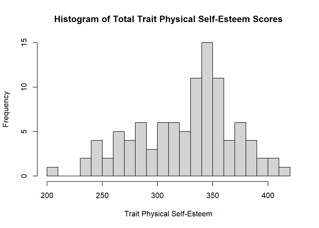
Create histograms for the other two conditions and comment on these.

2. Summary Statistics, Box Plot, Confidence Intervals (response)

2a. Summary Statistics

Task

Compare the summary statistics for the self esteem scores for TPSE, SPSE_1 and SPSE_2 to see if the rejection impacts on physical self esteem.

Previous Lesson

This is shown in Task 1a. of Property Section 7.0.2.

Using the summary statistics discuss the impact of the rejections on the self esteem scores.

Code

Code

#minimum value
apply(selfesteem[4:6],MARGIN=2,FUN=min) 

#maximum value
apply(selfesteem[4:6],MARGIN=2,FUN=max) 

Modify this code to also calculate the number of observations, means, and standard deviations.

Solution

Code

#minimum value
apply(selfesteem[4:6],MARGIN=2,FUN=min) 

  TPSE SPSE_1 SPSE_2 
   201    188     63 

Code

#maximum value
apply(selfesteem[4:6],MARGIN=2,FUN=max) 

  TPSE SPSE_1 SPSE_2 
   411    410    368 

Code

#number of observations
apply(selfesteem[4:6],MARGIN=2,FUN=length)

  TPSE SPSE_1 SPSE_2 
   100    100    100 

Code

#mean
apply(selfesteem[4:6],MARGIN=2,FUN=mean) 

  TPSE SPSE_1 SPSE_2 
325.91 317.97 198.79 

Code

#standard deviation
apply(selfesteem[4:6],MARGIN=2,FUN=sd) 

    TPSE   SPSE_1   SPSE_2 
44.16523 47.75748 66.31046 

Previous Lesson

See Task 1a. (Section 5.0.2) in Dolphins and Task 1a. (Section 7.0.2) in Property for examples of interpreting summary statistics.

2b. Box Plot

Task

Display the response variables TPSE, SPSE_1 and SPSE_2 graphically using the boxplot() function.

Previous Lesson

Dolphins 2a Section 5.0.3.

Using the box plot discuss the impact of the rejections on the self esteem scores.

Code

Code

boxplot(selfesteem$TPSE, selfesteem$SPSE_1, selfesteem$SPSE_2, data=selfesteem,main="Total Physical Self-Esteem Score by Condition",names=c("TPSE","SPSE1","SPSE2"))

Solution

Code

boxplot(selfesteem$TPSE, selfesteem$SPSE_1, selfesteem$SPSE_2, data=selfesteem,main="Total Physical Self-Esteem Score by Condition",names=c("TPSE","SPSE1","SPSE2"))

Previous Lesson

See Task 1a. (Section 3.0.2) in Cockles for interpretation of box plots.

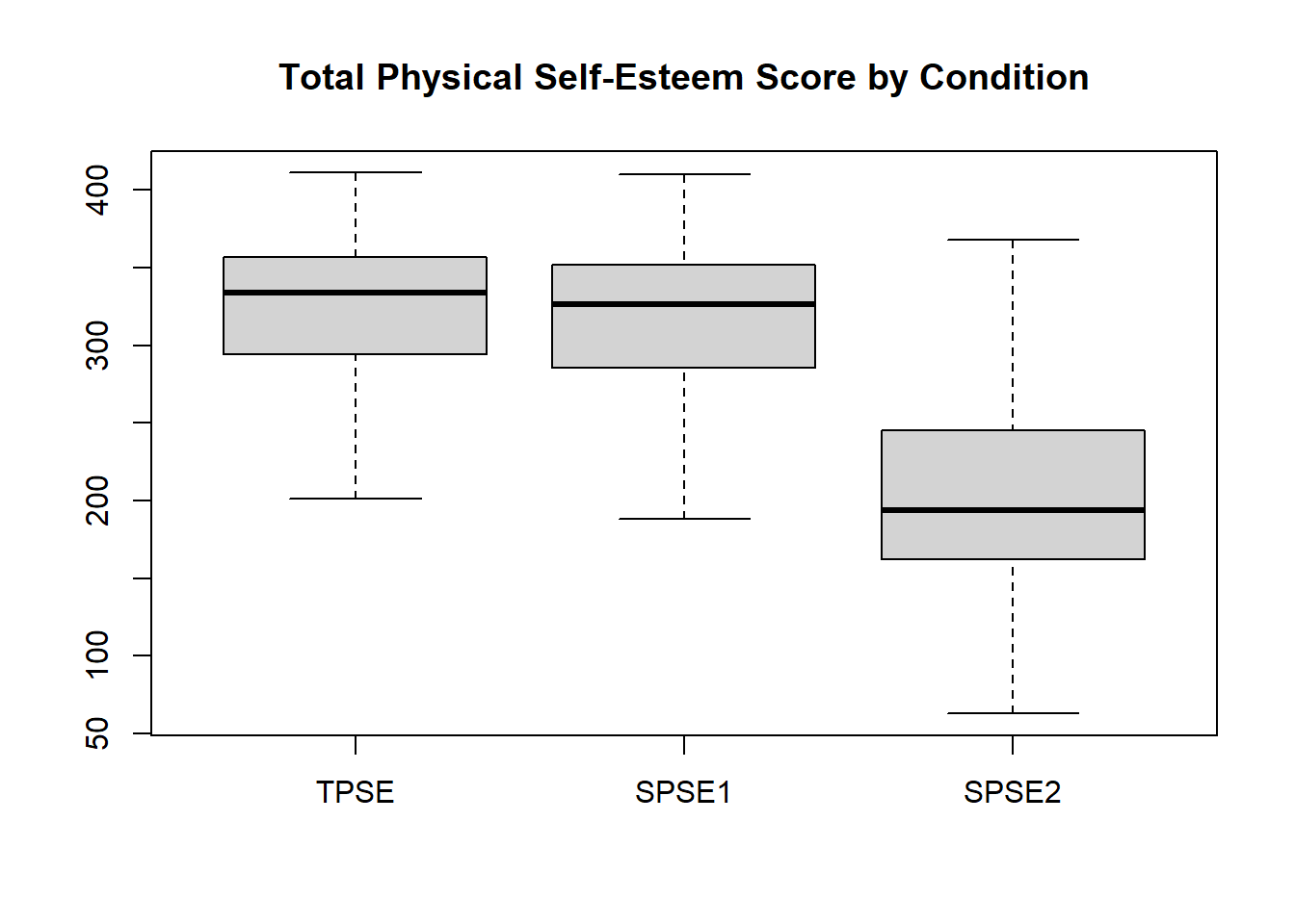
2c. Confidence Interval (paired difference)

Task

Calculate 95% confidence intervals for the differences in score between each pair of conditions (TPSE, SPSE_1 and SPSE_2), and report your findings.

Important Information

This can be achieved with a paired t.test().

Previous Lesson

Altitude Task 3 Section 6.0.4.

Code

Code

#first test if variances are equal
var.test(selfesteem$TPSE, selfesteem$SPSE_1, alternative = "two.sided") 

#no significant evidence against null hypothesis that variances are equal, use var.equal=T in t test
t.test(selfesteem$TPSE, selfesteem$SPSE_1,paired=T,var.equal=T,alternative="two.sided")

Solution

Code

#first test if variances are equal
var.test(selfesteem$TPSE, selfesteem$SPSE_1, alternative = "two.sided") 

    F test to compare two variances

data:  selfesteem$TPSE and selfesteem$SPSE_1
F = 0.85522, num df = 99, denom df = 99, p-value = 0.4379
alternative hypothesis: true ratio of variances is not equal to 1
95 percent confidence interval:
 0.5754281 1.2710579
sample estimates:
ratio of variances 
         0.8552207 

Code

#no significant evidence against null hypothesis that variances are equal, use var.equal=T in t test
t.test(selfesteem$TPSE, selfesteem$SPSE_1,paired=T,var.equal=T,alternative="two.sided")

    Paired t-test

data:  selfesteem$TPSE and selfesteem$SPSE_1
t = 2.6012, df = 99, p-value = 0.01071
alternative hypothesis: true mean difference is not equal to 0
95 percent confidence interval:
  1.883248 13.996752
sample estimates:
mean difference 
           7.94 

Previous Lesson

See Altitude Task 3 Section 6.0.4 for making conclusions from paired difference confidence intervals.

Extension

Compare the other combinations of conditions.

3. Summary Statistics, Box Plots, Confidence Intervals (response by predictor)

3a. Summary Statistics

Task

Compare the self esteem scores at each of the three conditions for males and females.

Important Information

This can be achieved using the function tapply().

Previous Lesson

Task 1a. in Dolphins Section 5.0.2.

Code

Code

#number of observations
tapply(selfesteem$TPSE,INDEX=selfesteem$Sex,FUN=length) 

#mean
tapply(selfesteem$TPSE,INDEX=selfesteem$Sex,FUN=mean) 

Modify this code to calculate the standard deviations, minimums and maximums of TPSE for each level of Sex.

Solution

Code

#number of observations
tapply(selfesteem$TPSE,INDEX=selfesteem$Sex,FUN=length) 

 1  2 
50 50 

Code

#mean
tapply(selfesteem$TPSE,INDEX=selfesteem$Sex,FUN=mean) 

     1      2 
310.98 340.84 

Code

#standard deviation
tapply(selfesteem$TPSE,INDEX=selfesteem$Sex,FUN=sd)

       1        2 
44.34443 38.98213 

Code

#minimum
tapply(selfesteem$TPSE,INDEX=selfesteem$Sex,FUN=min) 

  1   2 
201 235 

Code

#maximum
tapply(selfesteem$TPSE,INDEX=selfesteem$Sex,FUN=max) 

  1   2 
378 411 

Previous Lesson

See Task 1a. (Section 5.0.2) in Dolphins and Task 1a. (Section 7.0.2) in Property for examples of interpreting summary statistics.

Extension

Repeat for SPSE_1 and SPSE_2.

3b. Box Plot (long data)

Task

You can create a box plot of all 3 conditions for males vs. females at once, by converting the data into long format. The data is currently in wide format, with one row per participant and one column per physical self esteem score. This format makes it easy to get a good overview of the data set, however it reduces the range of models which can be fitted and can make plotting more complex.

Data in long format has a row for each observation (physical self esteem score) and a column for each variable (condition).

To convert the data from wide to long format, we use the tidyr package.

Previous Lesson

Install new packages using instructions in Getting started with R Section 2.6.

Previous Lesson

There is an example of wide to long data conversion and box plot construction in Task 2c. of Dolphins Section 5.0.3.

Discuss any visible patterns from the box plot, being sure to comment on any difference (or lack thereof) in self esteem scores for males and females on both an overall level as well as at each condition.

Code

The key that all our variables (e.g. TPSE,SPSE_1, etc) could be levels of is something like “Condition”, but note that you can use any key=” ” that makes sense.

The values of these variables are physical self esteem scores so we will call our second new column “PSE”, but again you can use any name that is sensible.

Select columns 4 to 6 of the original data set to gather into long format, leaving the Participant,Subject and Sex variables as unique columns as they are not a conditional physical self esteem score.

Code

library(tidyr)
selfesteemLong<-gather(data=selfesteem,key="Condition",value="PSE",4:6)

Create box plot of PSE against Sex and Condition

Code

boxplot(PSE~Sex*Condition,data=selfesteemLong,main="Total Physical Self-Esteem score by Condition and Sex",names=c("F:SPSE1","M:SPSE1","F:SPSE2","M:SPSE2","F:TPSE","M:TPSE"),ylab="Measurement")

Solution

The key that all our variables (e.g. TPSE,SPSE_1, etc) could be levels of is something like “Condition”, but note that you can use any key=” ” that makes sense.

The values of these variables are physical self esteem scores so we will call our second new column “PSE”, but again you can use any name that is sensible.

Select columns 4 to 6 of the original data set to gather into long format, leaving the Participant,Subject and Sex variables as unique columns as they are not a conditional physical self esteem score.

Code

library(tidyr)
selfesteemLong<-gather(data=selfesteem,key="Condition",value="PSE",4:6)

Code

boxplot(PSE~Sex*Condition,data=selfesteemLong,main="Total Physical Self-Esteem score by Condition and Sex",names=c("F:SPSE1","M:SPSE1","F:SPSE2","M:SPSE2","F:TPSE","M:TPSE"),ylab="Measurement")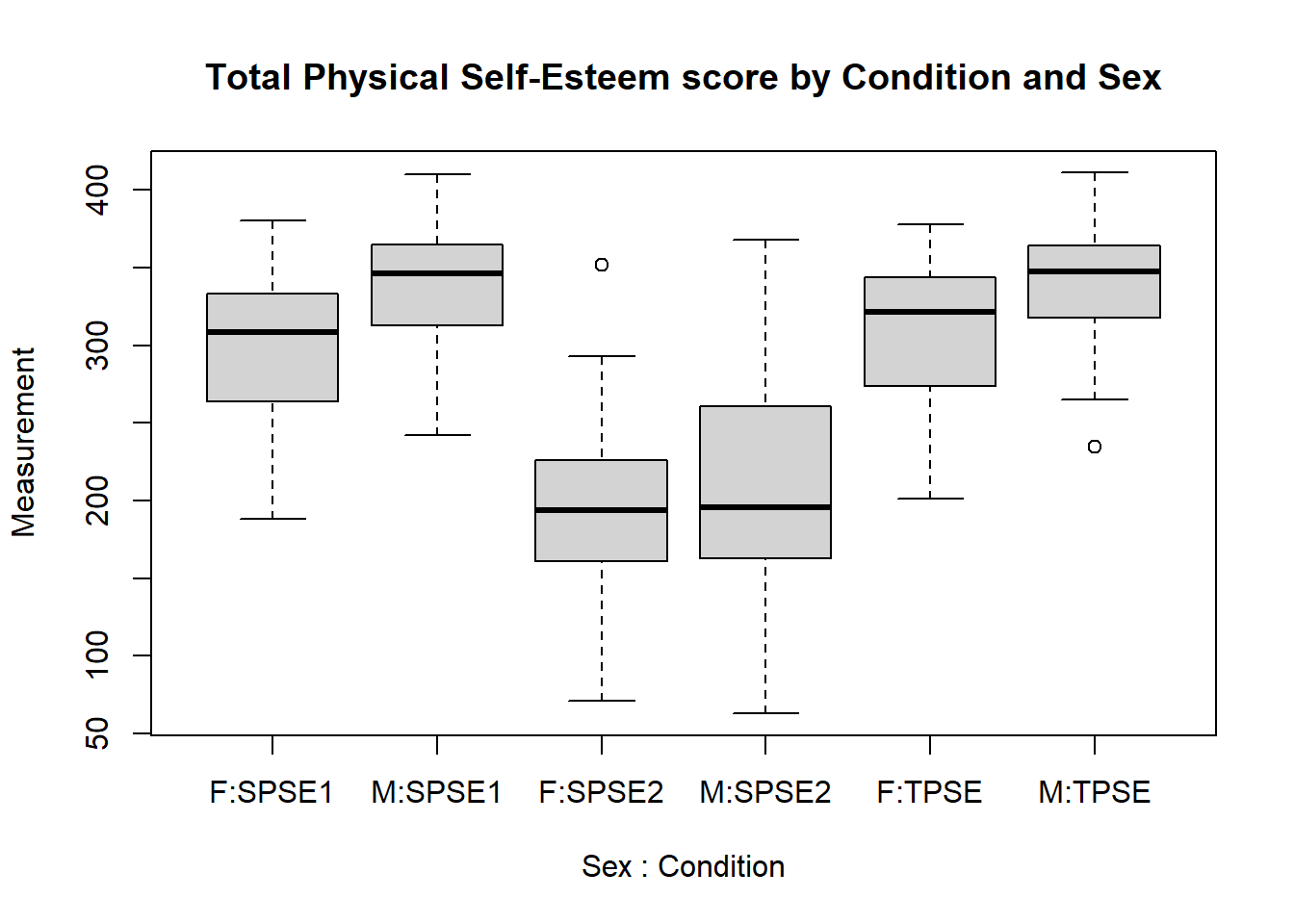

Previous Lesson

See Task 2a. (Section 3.0.3) in Cockles for interpretation of box plots with interactions between predictors.

3c. Confidence Intervals (difference in means)

Task

Construct 95% confidence intervals for the difference in mean scores according to Sex at each condition.

Important Information

These samples are no longer paired, as the males and females are different participants.

Previous Lesson

See Task 3b. of Cockles Section 3.0.4

Check for a significant difference in mean scores and report your findings.

Code

Code

#first test if variances are equal
var.test(selfesteem$TPSE[selfesteem$Sex=="1"], selfesteem$TPSE[selfesteem$Sex=="2"],alternative = "two.sided") 

#no significant evidence against null hypothesis that variances are equal, use var.equal=T in t test
t.test(selfesteem$TPSE[selfesteem$Sex=="1"],selfesteem$TPSE[selfesteem$Sex=="2"],paired=F,var.equal=T,alternative="two.sided")

Solution

Code

#first test if variances are equal
var.test(selfesteem$TPSE[selfesteem$Sex=="1"], selfesteem$TPSE[selfesteem$Sex=="2"],alternative = "two.sided") 

    F test to compare two variances

data:  selfesteem$TPSE[selfesteem$Sex == "1"] and selfesteem$TPSE[selfesteem$Sex == "2"]
F = 1.294, num df = 49, denom df = 49, p-value = 0.3701
alternative hypothesis: true ratio of variances is not equal to 1
95 percent confidence interval:
 0.7343356 2.2803384
sample estimates:
ratio of variances 
          1.294038 

Code

#no significant evidence against null hypothesis that variances are equal, use var.equal=T in t test
t.test(selfesteem$TPSE[selfesteem$Sex=="1"],selfesteem$TPSE[selfesteem$Sex=="2"],paired=F,var.equal=T,alternative="two.sided")

    Two Sample t-test

data:  selfesteem$TPSE[selfesteem$Sex == "1"] and selfesteem$TPSE[selfesteem$Sex == "2"]
t = -3.5761, df = 98, p-value = 0.0005437
alternative hypothesis: true difference in means is not equal to 0
95 percent confidence interval:
 -46.43009 -13.28991
sample estimates:
mean of x mean of y 
   310.98    340.84 

Previous Lesson

See Task 3b. of Cockles Section 3.0.4 for hypothesis test conclusions.

Extension

Carry out the same test for the SPSE_1 and SPSE_2 variables.

4. Extension: Summary Statistics, Box Plots, Confidence Intervals (response by predictor)

Extension

Using the methods shown to compare the male and female self esteem scores (e.g. summary statistics, box plots, 95% confidence intervals for difference in means), now compare the self esteem scores for PE students and non-PE students (Subject), and report your findings.

Previous Task

See Task 3 for code to modify.

5. New Variable, Extension: Summary Statistics, Box Plots (response)

5a. Calculate New Variable

Task

Calculate new variables Change_1 and Change_2 to measure the change in self-esteem scores after each rejection, e.g Change_1 is SPSE_1 score minus TPSE score.

Previous Lesson

This is similar to the creation of new variables in Property Task 4 Section 7.0.5.

Code

Code

selfesteem$Change_1<-selfesteem$SPSE_1-selfesteem$TPSE

Calculate Change_2 in the same way.

Solution

Code

selfesteem$Change_1<-selfesteem$SPSE_1-selfesteem$TPSE
selfesteem$Change_2<-selfesteem$SPSE_2-selfesteem$TPSE

5b. Extension: Summary Statistics, Box Plots

Extension

Discuss patterns in self esteem scores after rejection due to chance and incapability (Change_1 and Change_2), using box plots or summary statistics.

Previous Task

See Tasks 2a and 2b for code.

6. Summary Statistics, Bar Plot (response by predictor), Extension: Confidence Intervals (difference in means)

6a. Summary Tables

Task

Create tables that incorporate Subject into our analysis of Change_1 and Change_2.

Previous Task

See Task 3a for code.

Code

Code

#number of observations
tapply(selfesteem$Change_1,INDEX=selfesteem$Subject,FUN=length)

#mean
tapply(selfesteem$Change_1,INDEX=selfesteem$Subject,FUN=mean) 

Modify this code to calculate tables of standard deviations, minimums, and maximums.

Solution

Code

#number of observations
tapply(selfesteem$Change_1,INDEX=selfesteem$Subject,FUN=length) 

 1  2 
50 50 

Code

#mean
tapply(selfesteem$Change_1,INDEX=selfesteem$Subject,FUN=mean) 

     1      2 
-16.90   1.02 

Code

#standard deviation
tapply(selfesteem$Change_1,INDEX=selfesteem$Subject,FUN=sd)

       1        2 
35.63778 21.18094 

Code

#minimum
tapply(selfesteem$Change_1,INDEX=selfesteem$Subject,FUN=min) 

   1    2 
-183  -41 

Code

#maximum
tapply(selfesteem$Change_1,INDEX=selfesteem$Subject,FUN=max) 

 1  2 
54 85 

Previous Lesson

See Task 1a. (Section 5.0.2) in Dolphins and Task 1a. (Section 7.0.2) in Property for examples of interpreting summary statistics.

Extension

Carry out the same procedure for Change_2

6b. Bar Plot

Task

Make a bar plot showing the mean Change_1 and Change_2 for PE and non-PE students, using your results from 6a.

Code

Code

#constructing a matrix of the mean changes
PEMatrix<-matrix(c(-16.9,-132.74,1.02,-121.5),nrow=2,ncol=2)

Code

#barplot
#creating the bar plot. beside=TRUE groups the columns by the table rows (sex)
#names.arg gives the names of each column group
barplot(PEMatrix,beside=TRUE,names.arg=c("PE students","Non-PE students"), ylab="Mean Change",main="Change PSE score by Rejection type and PE/Non-PE student",col=rep(c("palegreen3","slateblue3"),2))

#legend
legend("topright",c("Chance Rejection","Non-chance Rejection"),fill=c("palegreen3","slateblue3"))

Solution

Code

#constructing a matrix of the mean changes
PEMatrix<-matrix(c(-16.9,-132.74,1.02,-121.5),nrow=2,ncol=2)

Code

#barplot
#creating the bar plot. beside=TRUE groups the columns by the table rows (sex)
#names.arg gives the names of each column group
barplot(PEMatrix,beside=TRUE,names.arg=c("PE students","Non-PE students"), ylab="Mean Change",main="Change PSE score by Rejection type and PE/Non-PE student",col=rep(c("palegreen3","slateblue3"),2))

legend("topright",c("Chance Rejection","Non-chance Rejection"),fill=c("palegreen3","slateblue3"))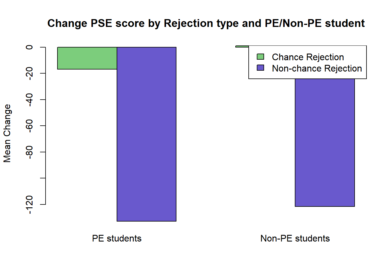

6c. Extension: Confidence Intervals (difference in means)

Extension

Calculate 95% confidence intervals and check if the changes in score Change_1 and Change_2 are significantly larger for a particular Subject (PE/non PE students).

Previous Task

Modify code from Task 3c.

7. Extension: Summary Statistics, Bar Plot, Confidence Intervals (response by predictor)

Extension

Repeat Task 6 to compare Change_1 and Change_2 by Sex.