8 Fiordland Rock Wren

A possible decrease in number of Rock Wren in the Fiordland area of New Zealand between 1985 and 2005 was investigated by the Department of Conservation. Numbers were recorded in 12 grids of 25 hectares at the two points in time. This research is presented by Ian Westbrooke.

Data

Data Summary

12 observations

3 variables

Variable	Type	Information
1984/85	Discrete	Count of rock-wren at each of 12 locations in 1984/85.
2005	Discrete	Count of rock-wren at each of 12 locations in 2005.
Change	Discrete	Difference in count between 2005 and 1984/85.

There is 1 data file associated with this presentation. It contains the data you will need to complete the lesson tasks.

Download Wren bird data.xls

Video

Objectives

Learning Objectives

New skills and concepts:

Jitter plot.
Add line to plot.

Reinforcing skills and concepts seen in earlier lessons:

Read data.
Summary statistics.
Strip chart.
Confidence interval and hypothesis test for mean, difference in means.
Bootstrap confidence interval.

Tasks

0. Read and Format data

0a. Read in the data

First check you have installed the package readxl (see Section 2.6) and set the working directory (see Section 2.1), using instructions in Getting started with R.

Load the data into R.

Important Information

Name your data wren for easier reference later.

Previous Lesson

To load the data in R we run code analogous to Task 0 in Cockles Section 3.0.1

The code has been hidden initially, so you can try to load the data yourself first before checking the solutions.

Code

library(readxl) #loads readxl package

wren<-read_xls("Wren bird data.xls") #loads the data file and names it wren

head(wren) #view beginning of data frame

Code

library(readxl) #loads readxl package

Warning: package 'readxl' was built under R version 4.2.2

Code

wren<-read_xls("Wren bird data.xls") #loads the data file and names it wren

head(wren) #view beginning of data frame

# A tibble: 6 × 3
  `1984/85` `2005` Change
      <dbl>  <dbl>  <dbl>
1         2      1     -1
2         1      1      0
3         1      1      0
4         1      0     -1
5         3      2     -1
6         3      1     -2

This opens a data frame containing 3 columns. 1984/85 is the number of rock wren counted at the 12 locations in the year 1985, 2005 is the counts in the same areas ten years later in 2005, and Change is the difference between the counts in 1985 and 2005.

1. Plot Data

1a. Scatter Plot

Construct a scatter plot of the 2005 count versus the 1984/85 count.

What do you notice about the data?

Code

plot(wren$`1984/85`,wren$`2005`,pch=18,col="green3",xlab="Count 1984/85",ylab="Count 2005",main = "Counts of Rock Wren in Fiordland")

Code

plot(wren$`1984/85`,wren$`2005`,pch=18,col="green3",xlab="Count 1984/85",ylab="Count 2005",main = "Counts of Rock Wren in Fiordland")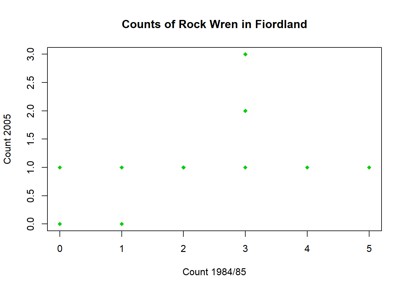

Some of the points lie directly on top of each other - there are 12 points in the data set but only 10 points showing in the graph.

1b. Scatter Plot with Jitter

Adding a small amount of variation (jitter) to one of the counts allows the overlapping points to be seen.

Jitter one of the variables, then use this to construct a new scatter plot.

A new column with the random variation can be produced using the jitter() function on the 1984/85 counts

Code

wren$Jitter1985<-jitter(wren$`1984/85`,factor=1.5)

Use this column to recreate the scatter plot, with added random jitter

Code

plot(wren$Jitter1985,wren$`2005`,pch=18,col="green3",xlab="Count 1984/85",ylab="Count 2005",main = "Counts of Rock Wren in Fiordland")

You can now see the two hidden points. The exact location of the points will vary for everyone as the jitter is random.

Code

#variable with random jitter
wren$Jitter1985<-jitter(wren$`1984/85`,factor=1.5)

plot(wren$Jitter1985,wren$`2005`,pch=18,col="green3",xlab="Count 1984/85",ylab="Count 2005",main = "Counts of Rock Wren in Fiordland")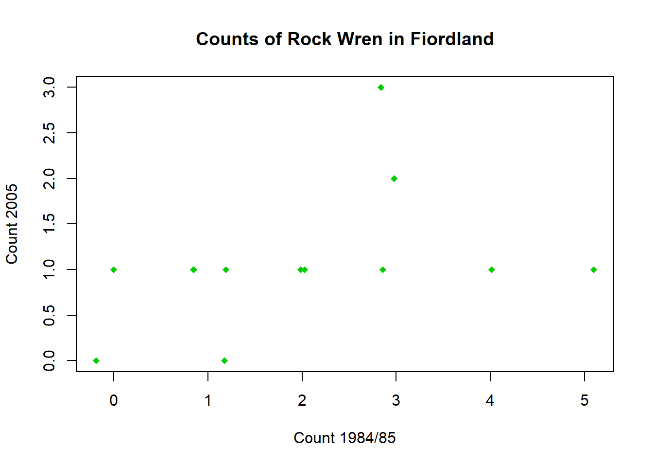

You should now see the two hidden points. The exact location of the points will vary for everyone as the jitter is random.

Produce the plot of Change versus 1984/85, with added jitter if necessary.

Does this show what’s happening in the data more clearly? Why or why not?

1c. Add Line

Add a 1-1 line to show the counts that would be expected if there was no change between 1984/85 and 2005.

Code

#repeat plot from Task 1a.
plot(wren$Jitter1985,wren$`2005`,pch=18,col="green3",xlab="Count 1984/85",ylab="Count 2005",main = "Counts of Rock Wren in Fiordland")

#add line with intercept 0 and slope 1
abline(0,1)

Code

#repeat plot from Task 1a.
plot(wren$Jitter1985,wren$`2005`,pch=18,col="green3",xlab="Count 1984/85",ylab="Count 2005",main = "Counts of Rock Wren in Fiordland")

#add line with intercept 0 and slope 1
abline(0,1)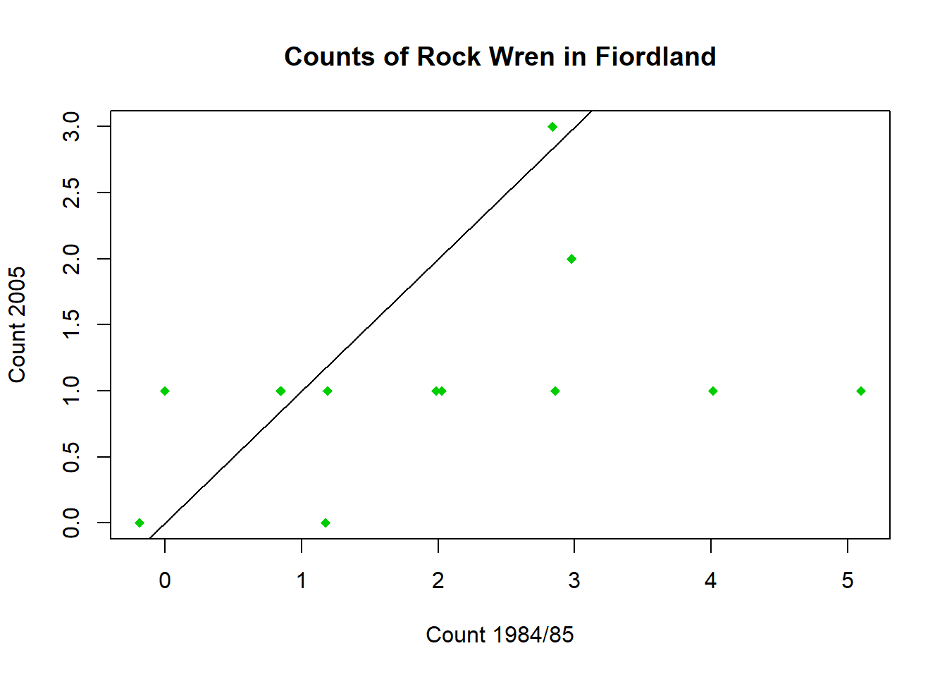

You can now see more clearly that most of the points are below the 1-1 line, indicating there were more birds in 1985 than 2005. Apart from the points that appear to be above due to jitter, only one point is actually above this line.

1d. Histogram

Draw a histogram of the Change column.

Code

hist(wren$Change,xlab="Change in count from 1984/85 to 2005",main="Change in Rock Wren count",breaks=6) #change breaks= to see distribution

Code

hist(wren$Change,xlab="Change in count from 1984/85 to 2005",main="Change in Rock Wren count",breaks=6) #change breaks= to see distribution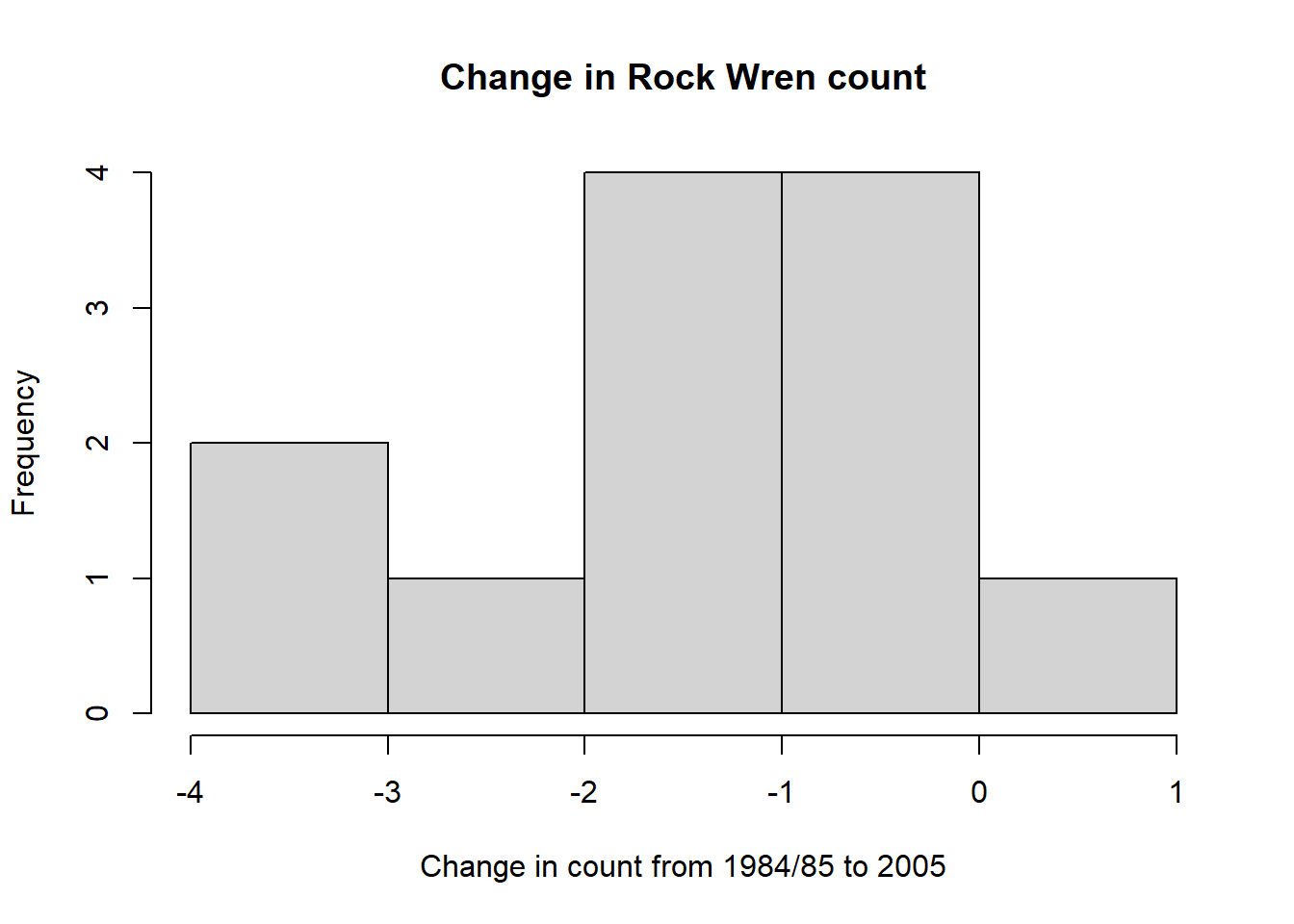

This shows only one of the changes in count was positive (greater than 0).

2. Summary Statistics, Strip Chart

2a. Summary Statistics

Compute and interpret the summary statistics for the columns.

Previous Lesson

See Task 1a. in Property Sales Section 7.0.2 for calculation of summary statistics by column.

Calculations for Change column are shown below.

Code

#mean
apply(wren[1:3],MARGIN=2,FUN=mean)

#median
apply(wren[1:3],MARGIN=2,FUN=median)

#standard deviation
apply(wren[1:3],MARGIN=2,FUN=sd)

Code

#mean
apply(wren[1:3],MARGIN=2,FUN=mean)

  1984/85      2005    Change 
 2.083333  1.083333 -1.000000

Code

#median
apply(wren[1:3],MARGIN=2,FUN=median)

1984/85    2005  Change 
      2       1      -1

Code

#standard deviation
apply(wren[1:3],MARGIN=2,FUN=sd)

  1984/85      2005    Change 
1.5642793 0.7929615 1.4142136

It can be seen that both the mean and median for Change (corresponding to the difference in means and medians between 1984/85 and 2005) is -1. Thus on average the number of rock wren decreased by one in each area over the ten years.

The larger standard deviation indicates there was more variation in the observed counts for 1984/85 compared to 2005.

2b. Strip Chart

Another way of viewing this data is with a dot-histogram, created using the stripchart() function in R. Plot the frequencies of each rock wren count for the years 1984/85 and 2005.

Previous Lesson

See Task 1. in Altitude Adjustment Section 6.0.2 for strip chart construction.

Code

stripchart(x=wren[,1:2],method="stack",vertical=T,pch=20,col="orange",offset=0.5,main="Rock Wren count frequencies")

Code

stripchart(x=wren[,1:2],method="stack",vertical=T,pch=20,col="orange",offset=0.5,main="Rock Wren count frequencies")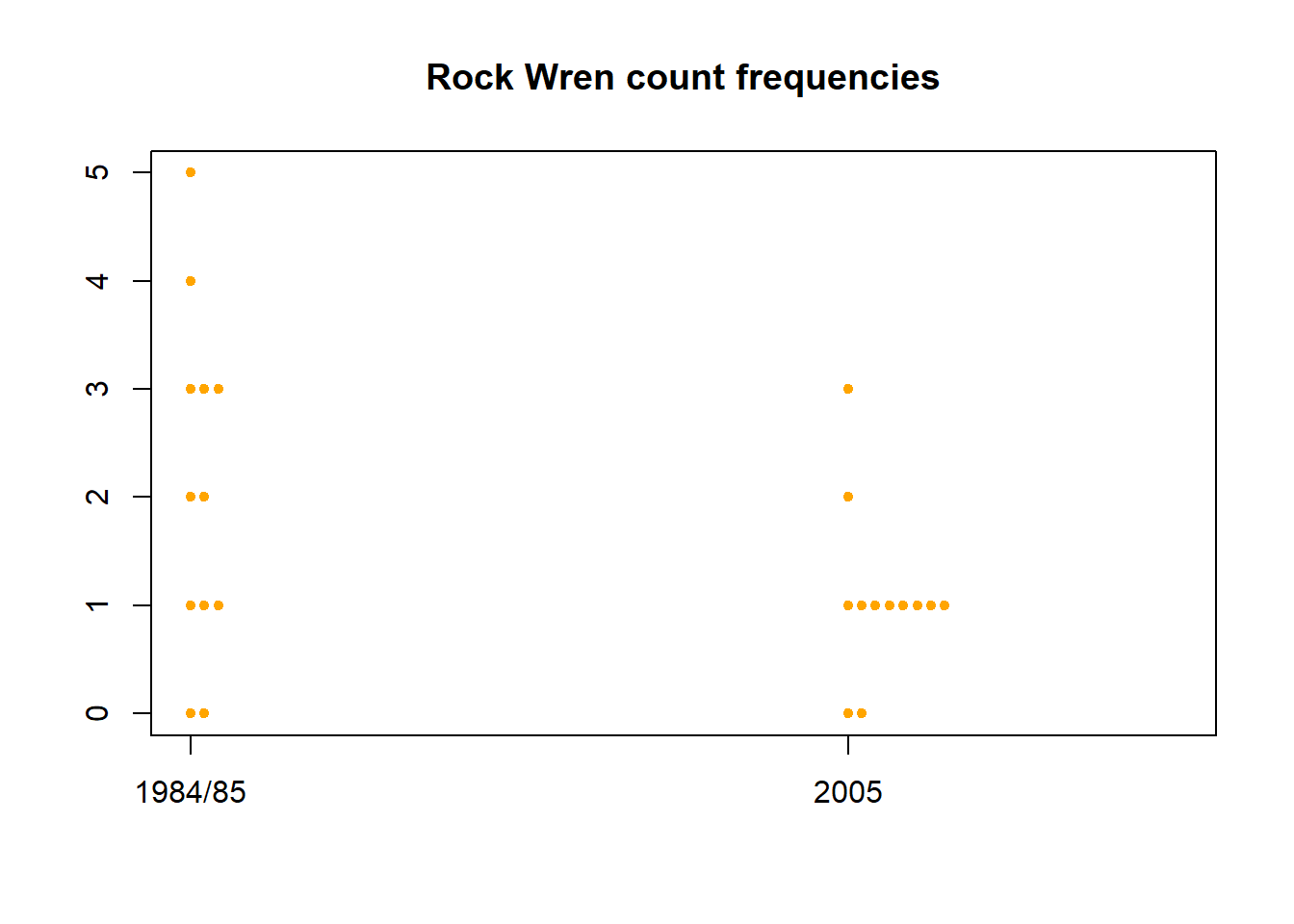

In 1984/85 there was greater variability in the rock wren counts, with over half the areas having counts of 2 or more and some having as many as 5. There was less variability in 2005, the vast majority of areas only had a count of 1 and the maximum observed count was 3.

3. Confidence Intervals, Hypothesis Tests (mean)

3a. Confidence Interval, Hypothesis Test (2-sided for mean)

We are interested in whether the decline in counts from 1985 to 2005 is more than could be expected by chance. Even if there was no change in the overall mean, sampling variation would lead to decreases in half the samples. The probability that a Change from 0 occurred by chance can be calculated by using a t-test.

Previous Lesson

Code from Task 1d. Cockles lesson Section 3.0.2 can be modified (subsetting not necessary).

Code

#alternative="two.sided" indicates we are interested in differences from 0 in any direction
t.test(wren$Change,alternative = "two.sided")

Code

#alternative="two.sided" indicates we are interested in differences from 0 in any direction
t.test(wren$Change,alternative = "two.sided")


    One Sample t-test

data:  wren$Change
t = -2.4495, df = 11, p-value = 0.03227
alternative hypothesis: true mean is not equal to 0
95 percent confidence interval:
 -1.8985484 -0.1014516
sample estimates:
mean of x 
       -1

It can be seen that the probability of this observed Change in wren numbers occurring by chance is 0.032, assuming there is no true change between 1985 and 2005. This probability is less than 1 in 20 (5%), and so is judged to be rare enough to be considered reasonable proof that there has been a significant change in the number of wren.

The confidence interval supports this conclusion as it is entirely less than 0. That, we can be 95% confidence that the true mean Change is negative.

3b. Confidence Interval, Hypothesis Test (1-sided for mean)

If we just testing for a decline in the numbers of wren, we could do a one-sided test that Change <0. Have a look at the help file for the t.test() function and modify the code from Task 3a. to test this.

What does this do to the probability?

Code

 #only interested in differences less than 0
t.test(wren$Change,alternative="less")

Code

 #only interested in differences less than 0
t.test(wren$Change,alternative="less")


    One Sample t-test

data:  wren$Change
t = -2.4495, df = 11, p-value = 0.01614
alternative hypothesis: true mean is less than 0
95 percent confidence interval:
       -Inf -0.2668331
sample estimates:
mean of x 
       -1

The probability of the observed Change in wren numbers occurring by chance is even lower now (assuming there is no true change between 1985 and 2005), giving greater proof that there has been a significant decrease in the observed number of wren.

3c. Confidence Interval, Hypothesis Test (mean difference)

A one sample t-test on the Change is equivalent to a two sample paired t-test using 1984/85 and 2005 as the variates. Confirm that this gives you the same results as the one sample analysis of change.

Previous Lesson

This is calculated in Task 3. of Altitude Adjustment Section 6.0.4.

Code

#first test if variances are equal
var.test(wren$`2005`,wren$`1984/85`, alternative = "two.sided") 

#significant evidence against null hypothesis that variances are equal, use var.equal=F in t test
t.test(wren$`2005`,wren$`1984/85`,paired=T,var.equal=F,alternative="two.sided")

Code

#first test if variances are equal
var.test(wren$`2005`,wren$`1984/85`, alternative = "two.sided")


    F test to compare two variances

data:  wren$`2005` and wren$`1984/85`
F = 0.25697, num df = 11, denom df = 11, p-value = 0.03337
alternative hypothesis: true ratio of variances is not equal to 1
95 percent confidence interval:
 0.07397473 0.89262236
sample estimates:
ratio of variances 
         0.2569659

Code

#significant evidence against null hypothesis that variances are equal, use var.equal=F in t test
t.test(wren$`2005`,wren$`1984/85`,paired=T,var.equal=F,alternative="two.sided")


    Paired t-test

data:  wren$`2005` and wren$`1984/85`
t = -2.4495, df = 11, p-value = 0.03227
alternative hypothesis: true mean difference is not equal to 0
95 percent confidence interval:
 -1.8985484 -0.1014516
sample estimates:
mean difference 
             -1

The p-value and confidence interval are identical to those calculated using a one-sample test on the Change variable.

4. Bootstrap Confidence Interval, Histogram (mean and median)

4a. Bootstrap Interval, Histogram (mean)

The t-test depends on the assumption that Change is normally distributed. To look whether the probability depends on this assumption, bootstrap resampling can be used.

Previous Lesson

You can modify code from Infrared Thermography Task 4 Section 4.1.5.

Do the bootstrap results support the t-test results?

Bootstrap for mean Change.

Code

library(boot)

#set seed so you get the same results when running again
set.seed(41)   

#function that calculates the mean from the bootstrapped samples
meanFun<-function(data,indices){  
  dataInd<-data[indices,]
  meandata<-mean(dataInd$Change)
  return(meandata)
}

#bootstrap mean change in counts
#create object called meanBoot with the output of the bootstrapping procedure
meanBoot<-boot(wren,statistic=meanFun, R=10000)

After running the bootstrap sampling, view summary statistics of the results by calling the output object.

Code

meanBoot

As an alternative to manual calculation of confidence intervals for the bootstrapped mean, we can use the boot.ci() function.

This returns a normal confidence interval (like those we have previously calculated by hand), along with percentile, basic, and accelerated bias-corrected intervals. The percentile interval method finds the 0.025 and 0.975 quantiles of our bootstrapped distribution and uses these as the lower and upper limits. This allows the interval to be skewed, removing the assumption of symmetry of the sampling distribution that the normal confidence interval requires. The basic and accelerated bias-corrected intervals are a bit more complicated, so we will not address them here. If you wish to learn more about then, you can check the references in the boot.ci() help file.

Code

boot.ci(meanBoot)

The advantage of boot.ci() is it allows both easy calculation and comparison of bootstrap confidence intervals. None of the intervals above contain the value zero, so it looks that the probability of this much change is less than 1 in 20.

Produce a histogram of the bootstrap means with the percentile confidence interval and median marked on top.

Code

percCi<-boot.ci(meanBoot,type="perc")

#check lower and upper limits from percentile interval object
percCi$percent[4:5]  

#calculate median
quantile(meanBoot$t,probs=0.5)

Code

#plot density histogram of bootstrap results
hist(meanBoot$t,breaks=12,freq=F,xlab="Mean Change in Counts", main="Bootstrap sample of Mean Change in Rock-Wren Counts") 

#add a smoothed line to show the distribution
lines(density(meanBoot$t), lwd = 2, col = "darkolivegreen3")

#add confidence limits
abline(v=c(quantile(meanBoot$t,probs=0.5),percCi$percent[4:5]),lty=2,col="darkolivegreen4")

Code

library(boot)

Warning: package 'boot' was built under R version 4.2.2

Code

#set seed so you get the same results when running again
set.seed(41)   

#function that calculates the mean from the bootstrapped samples
meanFun<-function(data,indices){  
  dataInd<-data[indices,]
  meandata<-mean(dataInd$Change)
  return(meandata)
}

#bootstrap mean change in counts
#create object called meanBoot with the output of the bootstrapping procedure
meanBoot<-boot(wren,statistic=meanFun, R=10000)

Code

meanBoot


ORDINARY NONPARAMETRIC BOOTSTRAP


Call:
boot(data = wren, statistic = meanFun, R = 10000)


Bootstrap Statistics :
    original      bias    std. error
t1*       -1 0.005783333   0.3857634

As an alternative to manual calculation of confidence intervals for the bootstrapped mean, we can use the boot.ci() function.

Code

boot.ci(meanBoot)

Warning in boot.ci(meanBoot): bootstrap variances needed for studentized
intervals

BOOTSTRAP CONFIDENCE INTERVAL CALCULATIONS
Based on 10000 bootstrap replicates

CALL : 
boot.ci(boot.out = meanBoot)

Intervals : 
Level      Normal              Basic         
95%   (-1.7619, -0.2497 )   (-1.7500, -0.2500 )  

Level     Percentile            BCa          
95%   (-1.7500, -0.2500 )   (-2.0000, -0.4167 )  
Calculations and Intervals on Original Scale

Code

percCi<-boot.ci(meanBoot,type="perc")

#check lower and upper limits from percentile interval object
percCi$percent[4:5]

[1] -1.75 -0.25

Code

#calculate median
quantile(meanBoot$t,probs=0.5)

50% 
 -1

Code

#plot density histogram of bootstrap results
hist(meanBoot$t,breaks=12,freq=F,xlab="Mean Change in Counts", main="Bootstrap sample of Mean Change in Rock-Wren Counts") 

#add a smoothed line to show the distribution
lines(density(meanBoot$t), lwd = 2, col = "darkolivegreen3")

#add confidence limits
abline(v=c(quantile(meanBoot$t,probs=0.5),percCi$percent[4:5]),lty=2,col="darkolivegreen4")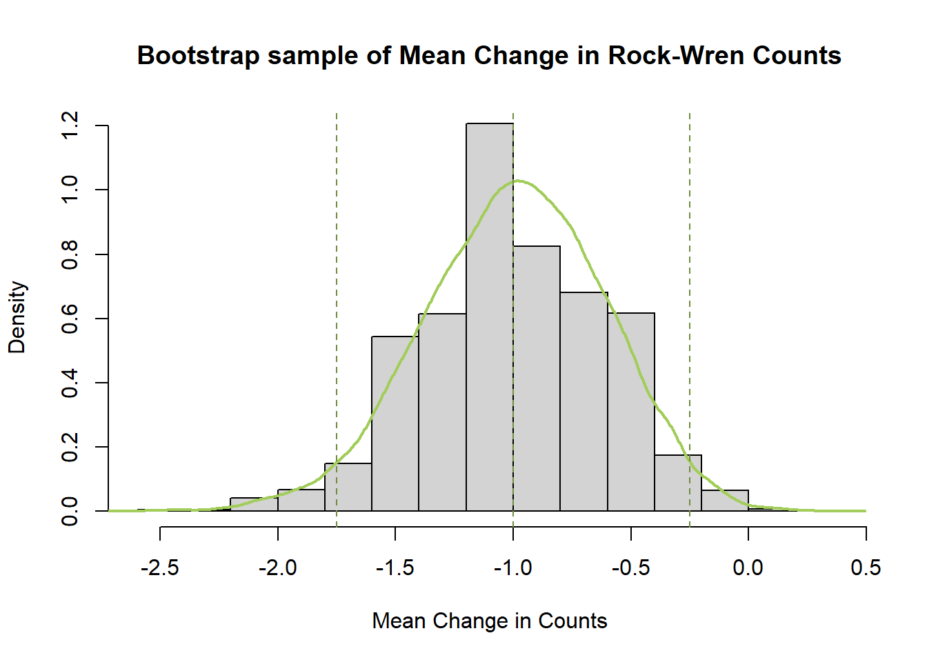

The bootstrapped means for the Change in rock wren counts follow a normal distribution symmetric around a mean of -1. This mean of means matches the one calculated earlier, and the distribution of bootstrapped mean estimates around it gives an indication of the amount of variability in our estimate due to sampling.

The bootstrap confidence interval is narrower than the one calculated earlier using t.test() and also includes only negative values so leads to the same conclusion. There is significant evidence to conclude the true change in counts from 1984/85 to 2005 has been negative.

As the earlier confidence interval was just below 0 and bootstrap confidence intervals can differ slightly from those calculated by hand or t.test() this outcome was not certain, but it is also not particularly unexpected.

The mean is more susceptible to being influenced by a single value. We could look at using the median and see how that looks under bootstrap resampling. Try changing the statistic to the median of the sample and boot strapping this.

Calculate the confidence limits using boot.ci(), and add an interval of your choice to the histogram of bootstrapped samples.

What do you notice about the confidence limits?

Why do you think the histogram looks like it does?

5. Confidence Interval, Hypothesis Test (unpaired data)

The test in Task 3c is a paired t-test as the 1984/85 and 2005 measurements were taken on the same grids. If the measurements in 2005 were taken on different grids randomly chosen we would need to do a two sample t-test.

Previous Task

Modify code from Task 3c.

How do these results compare with the paired t-test?

Code

#first test if variances are equal
var.test(wren$`2005`,wren$`1984/85`, alternative = "two.sided") 

#significant evidence against null hypothesis that variances are equal, use var.equal=F in t test
t.test(wren$`2005`,wren$`1984/85`,paired=F,var.equal=F,alternative="two.sided")

Code

#first test if variances are equal
var.test(wren$`2005`,wren$`1984/85`, alternative = "two.sided")


    F test to compare two variances

data:  wren$`2005` and wren$`1984/85`
F = 0.25697, num df = 11, denom df = 11, p-value = 0.03337
alternative hypothesis: true ratio of variances is not equal to 1
95 percent confidence interval:
 0.07397473 0.89262236
sample estimates:
ratio of variances 
         0.2569659

Code

#significant evidence against null hypothesis that variances are equal, use var.equal=F in t test
t.test(wren$`2005`,wren$`1984/85`,paired=F,var.equal=F,alternative="two.sided")


    Welch Two Sample t-test

data:  wren$`2005` and wren$`1984/85`
t = -1.9752, df = 16.303, p-value = 0.06543
alternative hypothesis: true difference in means is not equal to 0
95 percent confidence interval:
 -2.07163316  0.07163316
sample estimates:
mean of x mean of y 
 1.083333  2.083333

Comparing these results to those found using the paired t-test we find the p-value is no longer significant, indicating there is not enough evidence to reject the null hypothesis of no change in counts. The confidence interval supports this new conclusion as it is now wider and includes 0, meaning the true difference in mean counts could be negative or positive.

Taking measurements from the same grids reduces the impact of potential confounding variables (e.g. terrain type, food availability, water sources etc.) and enables us to make more accurate estimates and therefore detect true effects.

If the measurements were hypothetically taken on different grids (as illustrated in this task), the standard error corresponding to our estimates would be larger. This results in wider confidence intervals and reduced power to detect a true difference.

6. Bootstrap Confidence Interval, Histogram (difference in means)

We can also bootstrap the difference in means between the 1984/85 and 2005 samples.

Do these results support the two-sample test results?

How do they compare to the bootstrapped mean Change?

Previous Lesson

You can modify code from Infrared Thermography Task 6 Section 4.1.7.

Bootstrap difference in means

Code

library(boot)

#set seed so you get the same results when running again
set.seed(802)  

#function that calculates the difference in means from the bootstrapped samples
meandiffFun<-function(data,indices){  
  dataInd<-data[indices,]
  meandiff<-mean(dataInd$`2005`,na.rm=T)-mean(dataInd$`1984/85`,na.rm=T)
  return(meandiff)
}

#bootstrap difference in mean rock-wren counts between 1984/85 and 2005
#create object called meandiffBoot with the output of the bootstrapping procedure
meandiffBoot<-boot(wren,statistic=meandiffFun, R=10000)

Code

meandiffBoot

Calculate percentile confidence interval

Code

percCi<-boot.ci(meandiffBoot,type="perc")

#check lower and upper limits from percentile interval object
percCi$percent[4:5]  

#calculate median
quantile(meandiffBoot$t,probs=0.5)

Plot histogram of bootstrapped values, add percentile limits

Code

#plot density histogram of bootstrap results
hist(meandiffBoot$t,breaks=20,freq=F,xlab="Mean Change in Counts", main="Bootstrap sample of Mean Change in Rock-Wren Counts")  

#add a smoothed line to show the distribution
lines(density(meandiffBoot$t), lwd = 2, col = "darkolivegreen3") 

#add confidence limits
abline(v=c(quantile(meandiffBoot$t,probs=0.5),percCi$percent[4:5]),lty=2,col="darkolivegreen4")

Code

library(boot)

#set seed so you get the same results when running again
set.seed(802)  

#function that calculates the difference in means from the bootstrapped samples
meandiffFun<-function(data,indices){  
  dataInd<-data[indices,]
  meandiff<-mean(dataInd$`2005`,na.rm=T)-mean(dataInd$`1984/85`,na.rm=T)
  return(meandiff)
}

#bootstrap difference in mean rock-wren counts between 1984/85 and 2005
#create object called meandiffBoot with the output of the bootstrapping procedure
meandiffBoot<-boot(wren,statistic=meandiffFun, R=10000)

Code

meandiffBoot


ORDINARY NONPARAMETRIC BOOTSTRAP


Call:
boot(data = wren, statistic = meandiffFun, R = 10000)


Bootstrap Statistics :
    original   bias    std. error
t1*       -1 0.002475   0.3878805

Code

percCi<-boot.ci(meandiffBoot,type="perc")

#check lower and upper limits from percentile interval object
percCi$percent[4:5]

[1] -1.833333 -0.250000

Code

#calculate median
quantile(meandiffBoot$t,probs=0.5)

50% 
 -1

Code

#plot density histogram of bootstrap results
hist(meandiffBoot$t,breaks=20,freq=F,xlab="Mean Change in Counts", main="Bootstrap sample of Mean Change in Rock-Wren Counts")  

#add a smoothed line to show the distribution
lines(density(meandiffBoot$t), lwd = 2, col = "darkolivegreen3") 

#add confidence limits
abline(v=c(quantile(meandiffBoot$t,probs=0.5),percCi$percent[4:5]),lty=2,col="darkolivegreen4")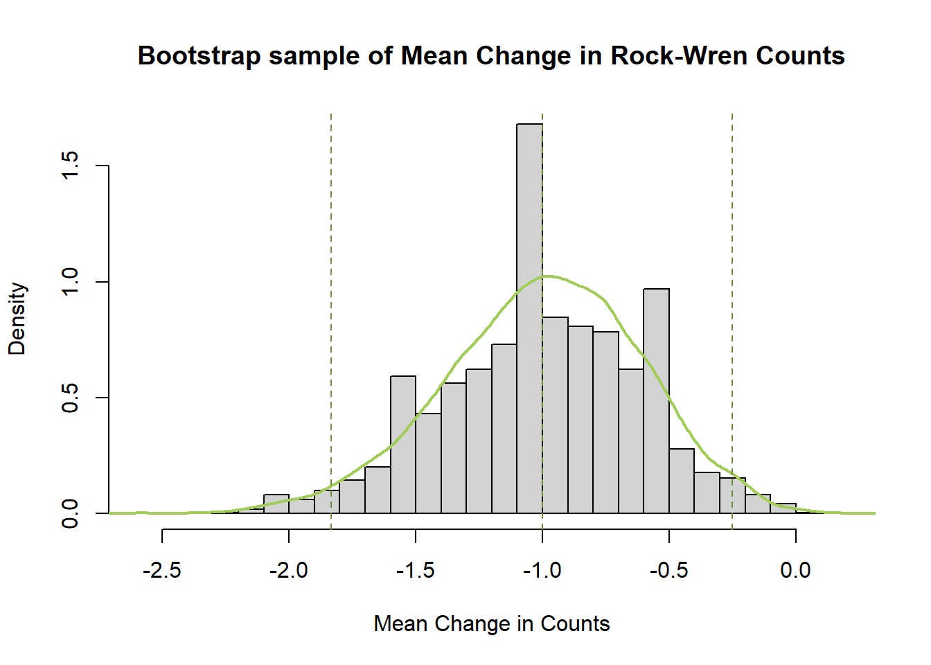

The bootstrapped difference in mean rock wren counts between 1984/85 and 2005 follows a normal distribution symmetric around a mean of -1. This mean of the difference in means matches the one calculated earlier, and the distribution of bootstrapped difference in mean estimates around it gives an indication of the amount of variability in our estimate due to sampling.

The bootstrap confidence interval is narrower than the one calculated by the two-sample t.test(), only including negative values and leading to a difference conclusion. There is significant evidence to conclude the true difference in mean counts from 1984/85 to 2005 has been negative.

Compared to the bootstrap for mean Change in rock wren counts (paired difference) this percentile interval is slightly wider (expected due to increased error from grid variability) but leads to the same conclusion of a decrease in counts.

Repeat the bootstrap procedure for the difference in medians.