12 Otago Stadium
We have a survey open right now that we invite you to fill out.
Support (or lack of support) from the Otago community to use public funding to construct the new Otago stadium, Forsyth Barr Stadium, was widely discussed and debated for some time. A survey questionnaire about this topic was distributed to 5000 residents in Dunedin city, New Zealand. Responses were received from 2248 residents.This lesson investigates the factors that influenced residents support for public funding of the stadium. The study was carried out by John Williams (Department of Marketing, University of Otago).
Data
There is 1 file associated with this presentation. It contains the data you will need to complete the lesson tasks.
Video
Objectives
Tasks
0. Read data
0a. Read in the data
First check you have installed the package readxl (see Section 2.6) and set the working directory (see Section 2.1), using instructions in Getting started with R.
Load the data into R.
This opens a data frame from a study investigating what proportion of residents support using public funds to construct the new Otago Stadium (note that this means support public funding of the stadium, not support the stadium).
The code has been hidden initially, so you can try to load the data yourself first before checking the solutions.
Code
#loads readxl package
library(readxl)

#loads the data file and names it stadium
stadium<-read_xls("stadiumreduced.xls")

#view beginning of data frame
head(stadium)
Code
#loads readxl package
library(readxl)
Warning: package 'readxl' was built under R version 4.2.2Code
#loads the data file and names it stadium
stadium<-read_xls("stadiumreduced.xls")

#view beginning of data frame
head(stadium)
# A tibble: 6 × 9
Support Age Employment Education AgeGroup HomeOwn Ratepayer income sex
<dbl> <dbl> <dbl> <dbl> <dbl> <dbl> <dbl> <dbl> <dbl>
1 1 27 6 7 2 3 1 5 1
2 2 28 6 7 2 2 1 3 1
3 2 29 6 7 2 1 0 5 1
4 2 31 6 7 2 2 1 3 1
5 3 35 6 7 3 2 1 NA 1
6 2 36 6 7 3 2 1 2 1We are using a simplified data frame with 1950 respondents. The full data set was cleaned up by removing a number of variables used in the data entry, removing cases where there were missing values and removing the five cases under 20. Consequently the results from the following tasks may differ slightly from those in the video.
The variables recorded are Support (Do you support public funding of the Otago Stadium? 1=Yes, 2=No, 3=Undecided), Age (age of respondent), Employment (employment situation), Education, AgeGroup (categorical age group of respondent), HomeOwn (living situation), Ratepayer (1=Yes, 0=No), income (cateogrical income bracket) and sex (1=Female, 0=Male).
1. Calculation, Confidence Interval (proportion)
1a. Proportion Calculation
The first step of the analysis is to calculate the (crude) proportion of respondents that do not support public funding for the stadium (Support=2 response category).
Crude proportions can be calculated manually from a table of counts by category using table() with margins (sums) added. Try to modify code from previous lessons to create this.
Code
#note we can apply to the addmargins() function directly to our table
addmargins(table(stadium$Support,dnn=c("Support")))
Proportions can also be found directly using the prop.table() function.
Code
#calculate proportion from table using prop.table
prop.table(table(stadium$Support,dnn=c("Support")))
Crude proportions can be calculated manually from a table of counts by category.
Code
#note we can apply to the addmargins() function directly to our table
addmargins(table(stadium$Support,dnn=c("Support")))
Support
1 2 3 Sum
530 1290 130 1950 Code
support1<-530/1950
support2<-1290/1950
support3<-130/1950
Proportions can also be found directly using the prop.table() function.
Code
#calculate proportion from table using prop.table
prop.table(table(stadium$Support,dnn=c("Support")))
Support
1 2 3
0.27179487 0.66153846 0.06666667 1b. Confidence Interval (proportion)
Construct a 95% confidence interval for the proportion who do not support public funding.
Interpret this confidence interval in terms of the number of respondents that do not support public funding of the Otago Stadium.
Although the procedure for calculating these kinds of confidence intervals by hand is covered in the video, we will instead use the prop.test() function as this is much more efficient.
You could repeat these questions calculating the confidence intervals manually if you wish (note you may get slightly different results, you can have a look at the prop.test() help file to see why this is, but the conclusions should be the same).
Code
#first argument is the number of successes (in this case having a particular opinion on the stadium)
#second argument is number of trials (all respondents to Support)
#note the use of length to sum the counts
prop.test(length(which(stadium$Support=="2")),n=length(stadium$Support))
Code
#first argument is the number of successes (in this case having a particular opinion on the stadium)
#second argument is number of trials (all respondents to Support)
#note the use of length to sum the counts
prop.test(length(which(stadium$Support=="2")),n=length(stadium$Support))
    1-sample proportions test with continuity correction

data:  length(which(stadium$Support == "2")) out of length(stadium$Support), null probability 0.5
X-squared = 202.89, df = 1, p-value < 2.2e-16
alternative hypothesis: true p is not equal to 0.5
95 percent confidence interval:
 0.6399772 0.6824567
sample estimates:
        p
0.6615385 2. Cross-Tabulation, Bar Plot (response by predictor)
2a. Cross-Tabulation
Construct a cross tabulation of sex against each of the categories in Support (No, Yes and Undecided).
We don’t need to worry about margins or proportions for this table, as we are only interested in counts for our bar plot.
Code
#title vector now has 2 entries
#specified in the same order the variables were provided to the table function
table(stadium$sex,stadium$Support,dnn=c("Sex","Support"))
Code
#calculate table without labels to supply heights to bars
stadiumMatrix<-table(stadium$sex,stadium$Support)
Code
#title vector now has 2 entries
#specified in the same order the variables were provided to the table function
table(stadium$sex,stadium$Support,dnn=c("Sex","Support"))
Support
Sex 1 2 3
0 309 639 48
1 221 651 82Code
#calculate table without labels to supply heights to bars
stadiumMatrix<-table(stadium$sex,stadium$Support)
2b. Bar Plot
Use your table from 2a. to create a bar plot.
Try adding some bells and whistles (e.g. colour, a legend) to make it more attractive.
What tentative conclusions can you make from this bar chart?
Code
#specify colour of bars by sex and support using a vector that repeats the 2 colours 3 times
barplot(stadiumMatrix,beside=TRUE,names.arg=c("Yes","No","Undecided"),ylab="Count", xlab="Support public funding",main="Support for public funding of the Dunedin stadium by sex",col=rep(c("royalblue4","goldenrod1"),3))

#legend, colours provided in boxes using fill=c()
legend("topright",c("Male","Female"),fill=c("royalblue4","goldenrod1"))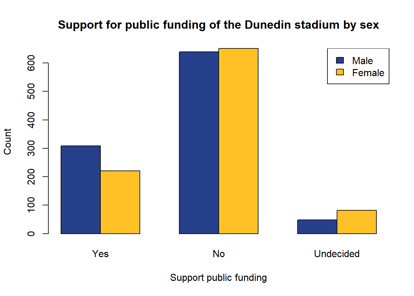
Of the people surveyed, those who supported publicly funding the stadium were more likely to be male than female while those who were undecided were more likely to be female. There were slightly more females than males who did not support the stadium.
3. Confidence Intervals (difference in proportions)
Set up confidence intervals for the difference between the proportions of men and women (sex) in the three Support categories (No, Undecided and Yes).
Interpret this confidence interval and state any conclusions you can make.
The hidden code shows the calculation of the difference between proportions of men and women who do not support public funding of the stadium (Support=2).
Code
#first argument is the number of successes (in this case not supporting the stadium),
#second argument is number of trials
prop.test(c(length(which(stadium$sex=="1"&stadium$Support=="2")),length(which(stadium$sex=="0"&stadium$Support=="2"))),
n=c(length(which(stadium$sex=="1")),length(which(stadium$sex=="0"))))
    2-sample test for equality of proportions with continuity correction

data:  c(length(which(stadium$sex == "1" & stadium$Support == "2")), length(which(stadium$sex == "0" & stadium$Support == "2"))) out of c(length(which(stadium$sex == "1")), length(which(stadium$sex == "0")))
X-squared = 3.4468, df = 1, p-value = 0.06337
alternative hypothesis: two.sided
95 percent confidence interval:
 -0.00215057  0.08379791
sample estimates:
   prop 1    prop 2
0.6823899 0.6415663 Calculate confidence intervals for the difference in the proportions of men and women who selected a) “undecided” (Support=3) and b) “Yes” (Support=1) for their support of public funding for the stadium.
Interpret your confidence intervals.
4. Extension: Cross-Tabulations, Bar Plots, Confidence Intervals (response by predictor)
4a. Age Group and Support
Construct a cross tabulation of AgeGroup against Support, and create a bar graph showing this information.
Calculate the confidence interval for difference between the proportion of respondents aged “25-34” and “55-64” that answered “No” in support for public funding for the stadium.
Interpret your result.
4b. Income and Support
Construct a cross tabulation of income against Support, and create a bar graph showing this information (with income as the factor on the x-axis and Support as the grouping variable).
Calculate the confidence interval for the difference between the proportion of respondents with income “<$30,000” and “>$100,000” that answered “No” in support for public funding for the stadium. Interpret your confidence interval.
4c. Rate-Paying Status and Support
Construct a cross tabulation of Ratepayer against Support, and create a bar graph showing this information (with Ratepayer as the factor for the x-axis and Support as the grouping variable).
Calculate the confidence interval for the difference between the proportion of respondents who were ratepayers and those who were not ratepayers that answered “No” in support of public funding for the stadium.
Interpret your confidence interval.
4d. Independent Exploration
Construct cross-tabulations and bar plots, and calculate any other appropriate confidence intervals for difference between proportions.
5. New Variable, Logistic Regression
Carry out a logistic regression with a binary variable that indicates support yes or no for the stadium as the response and sex, income and Age as predictor variables.
Write out the logistic regression model and report any conclusions.
First create a new variable No (support for the stadium yes/no recoded as 0/1, note that “undecided” is coded as 0 for illustrative purposes only)
Code
#vector of zeros the length of the data set, place holder
stadium$No <-c(rep(0,length=nrow(stadium)))

#replace instances corresponding to support=No with 1s
stadium$No[stadium$Support=="2"]<-1
Specify income as a factor variable
Code
stadium$income<-as.factor(stadium$income)Use the glm() function to fit a generalised linear model in R. By specifying the family as binomial (binary response) with a logit link a logistic regression is performed.
Code
supportModel<-glm(No~sex+income+Age,data=stadium,family=binomial(link="logit"))
summary(supportModel)
anova(supportModel,test="Chisq")
Code
#vector of zeros the length of the data set, place holder
stadium$No <-c(rep(0,length=nrow(stadium)))

#replace instances corresponding to support=No with 1s
stadium$No[stadium$Support=="2"]<-1
Code
stadium$income<-as.factor(stadium$income)Code
supportModel<-glm(No~sex+income+Age,data=stadium,family=binomial(link="logit"))
summary(supportModel)
Call:
glm(formula = No ~ sex + income + Age, family = binomial(link = "logit"),
    data = stadium)

Deviance Residuals:
    Min       1Q   Median       3Q      Max
-1.7450  -1.3344   0.7474   0.9720   1.2362

Coefficients:
             Estimate Std. Error z value Pr(>|z|)
(Intercept)  0.987886   0.251789   3.923 8.73e-05 ***
sex          0.113404   0.100963   1.123    0.261
income2     -0.205547   0.153446  -1.340    0.180
income3     -0.676523   0.162327  -4.168 3.08e-05 ***
income4     -0.699557   0.164311  -4.258 2.07e-05 ***
income5     -1.164967   0.162463  -7.171 7.46e-13 ***
Age          0.001904   0.003399   0.560    0.575
---
Signif. codes:  0 '***' 0.001 '**' 0.01 '*' 0.05 '.' 0.1 ' ' 1

(Dispersion parameter for binomial family taken to be 1)

    Null deviance: 2427.7  on 1886  degrees of freedom
Residual deviance: 2347.0  on 1880  degrees of freedom
  (63 observations deleted due to missingness)
AIC: 2361

Number of Fisher Scoring iterations: 4
Code
anova(supportModel,test="Chisq")Analysis of Deviance Table
Model: binomial, link: logit
Response: No
Terms added sequentially (first to last)
Df Deviance Resid. Df Resid. Dev Pr(>Chi)
NULL 1886 2427.7
sex 1 4.273 1885 2423.4 0.03873 *
income 4 76.133 1881 2347.3 1.148e-15 ***
Age 1 0.313 1880 2347.0 0.57561
---
Signif. codes: 0 '***' 0.001 '**' 0.01 '*' 0.05 '.' 0.1 ' ' 1The regression equation for the fitted model may be written as follows
\[ \log \frac{p}{(1-p)} = 0.9879 + 0.1134_{SEX} - 0.2055_{INCOME2} - 0.6765_{INCOME3} - 0.6996_{INCOME4} -1.1650_{INCOME5} + 0.0019_{AGE} \] where \(p\) is the probability of not supporting publicly funding the Otago stadium.
For females (sex=1) the odds of not supporting the stadium is increased by a multiplicative factor of \(exp( 0.113404) = 1.1201\) compared to males, although with a p-value of 0.261 this is not a significant effect. Respondent age is also not significantly related to not supporting the stadium, the estimate is for each one year increase in age, the odds of not supporting the stadium increase by a multiplicative factor of \(exp(0.001904) = 1.0019\). There are significant effects of most income brackets relative to the lowest one. The estimates for their effect on log-odds of not supporting the stadium are increasingly negative (for greater income), which corresponds to larger decreases in the odds of not supporting the stadium (multiplicative factor <1) compared to respondents in the lowest income bracket.
The analysis of deviance chi-squared values for the sex and income variables are less than 0.05, indicating a significant increase in deviance if these were removed from the model. However the Age variable has a non-significant p-value of 0.5756, so should be removed from the model in the interests of parsimony (fitting the best model with as few parameters as possible).
6. Multiple Logistic Regression
Carry out a multinomial logistic regression with Support (Yes, No and Undecided) as the outcome variable and sex,income and Age as predictors.
Make sure to first install the package mlogit using instructions in Getting started with R Section 2.6.
The format for specifying our mlogit() model is similar to that used for logistic regression, but with a couple of key differences. This function has the flexibility to include both “alternative-specific” and “individual-specific” predictor variables, which are given to the left (alternative) and right (individual) of the | sign. Since we only have individual-specific predictors, we provide these on the right side of the |, and put a 0 on the left side. We also must indicate that our data is in “wide” format.
Report your conclusions from the fitted model. The fitted models for multinomial logistic regression may be written out and interpreted using methods analogous to logistic regression. However, because there are now more than 2 response categories, we must construct several fitted equations for the comparison of each set of log-odds.
Code
library(mlogit)
multiModel<-mlogit(Support~0|sex+income+Age,data=stadium,shape="wide")
summary(multiModel)
The Support variable has 3 levels : 1=Yes, 2=No, 3=Undecided. The reference category in the multinomial model above is Support=1. The fitted equation for the log-odds of not supporting the stadium relative to supporting the stadium is written using the model parameters with “:2” after them.
\[\log\left(\frac{No}{Yes}\right) = 1.4720 + 0.2549_{\text{Sex}} - 0.3335 _{\text{Income2}} - 0.8542 _{\text{Income3}} - 0.9347 _{\text{Income4}} - 1.4289 _{\text{Income5}} - 0.0011_{\text{Age}}\] Write out the fitted equation for the log-odds of being undecided relative to supporting the stadium, using the model parameters with “:3” after them.
To find the log-odds of not supporting the stadium relative to being undecided, we make use of the above 2 fitted equations and the following log rule.
\[\log\left(\frac{a}{b}\right) = \log(a) - \log(b)\] \[\log\left(\frac{No}{Undecided}\right) = \log\left(\frac{No/Yes}{Undecided/Yes}\right) = \log\left(\frac{No}{Yes}\right) - \log\left(\frac{Undecided}{Yes}\right)\] Use this derivation to calculate the fitted equation for the log-odds of not supporting the stadium relative to being undecided.
Code
library(mlogit)Loading required package: dfidx
Attaching package: 'dfidx'The following object is masked from 'package:stats':
filterCode
multiModel<-mlogit(Support~0|sex+income+Age,data=stadium,shape="wide")
summary(multiModel)
Call:
mlogit(formula = Support ~ 0 | sex + income + Age, data = stadium,
    shape = "wide", method = "nr")

Frequencies of alternatives:choice
       1        2        3
0.276100 0.656598 0.067303

nr method
6 iterations, 0h:0m:0s
g'(-H)^-1g = 4.62E-06
successive function values within tolerance limits

Coefficients :
                Estimate Std. Error z-value  Pr(>|z|)
(Intercept):2  1.4720274  0.2820258  5.2195 1.794e-07 ***
(Intercept):3 -0.4396044  0.4825230 -0.9111 0.3622671
sex:2          0.2548934  0.1097484  2.3225 0.0202047 *
sex:3          0.7052770  0.2072019  3.4038 0.0006645 ***
income2:2     -0.3335363  0.1729407 -1.9286 0.0537784 .
income2:3     -0.4774254  0.3035085 -1.5730 0.1157138
income3:2     -0.8542089  0.1808314 -4.7238 2.315e-06 ***
income3:3     -0.7017248  0.3143475 -2.2323 0.0255937 *
income4:2     -0.9346950  0.1816450 -5.1457 2.665e-07 ***
income4:3     -1.0272698  0.3346487 -3.0697 0.0021428 **
income5:2     -1.4289235  0.1784917 -8.0055 1.110e-15 ***
income5:3     -1.2344975  0.3256521 -3.7908 0.0001501 ***
Age:2         -0.0011040  0.0037578 -0.2938 0.7689071
Age:3         -0.0129463  0.0066451 -1.9482 0.0513857 .
---
Signif. codes:  0 '***' 0.001 '**' 0.01 '*' 0.05 '.' 0.1 ' ' 1

Log-Likelihood: -1476.7
McFadden R^2:  0.03762
Likelihood ratio test : chisq = 115.45 (p.value = < 2.22e-16)
The Support variable has 3 levels : 1=Yes, 2=No, 3=Undecided. The reference category in the multinomial model above is Support=1. The fitted equation for the log-odds of not supporting the stadium relative to supporting the stadium is written using the model parameters with “:2” after them.
\[\log\left(\frac{No}{Yes}\right) = 1.4720 + 0.2549_{\text{Sex}} - 0.3335 _{\text{Income2}} - 0.8542 _{\text{Income3}} - 0.9347 _{\text{Income4}} - 1.4289 _{\text{Income5}} - 0.0011_{\text{Age}}\] Write out the fitted equation for the log-odds of being undecided relative to supporting the stadium, using the model parameters with “:3” after them.
\[\log\left(\frac{Undecided}{Yes}\right) = - 0.4396 + 0.7053_{\text{Sex}} - 0.4774 _{\text{Income2}} - 0.7017 _{\text{Income3}} - 1.0273 _{\text{Income4}} - 1.2345 _{\text{Income5}} - 0.0129_{\text{Age}}\]
\[\log\left(\frac{No}{Undecided}\right) = \log\left(\frac{No/Yes}{Undecided/Yes}\right) = \log\left(\frac{No}{Yes}\right) - \log\left(\frac{Undecided}{Yes}\right)\] Use this derivation to calculate the fitted equation for the log-odds of not supporting the stadium relative to being undecided.
\[\log\left(\frac{No}{Undecided}\right) = 1.9116 - 0.4504_{\text{Sex}} + 0.1439_{\text{Income2}} - 0.1525 _{\text{Income3}} + 0.0926 _{\text{Income4}} - 0.1944_{\text{Income5}} + 0.0118_{\text{Age}}\]
7. Extension: Post-Stratification
Post-stratification is the process of calculating separate estimates of a response for each value of a certain predictor variable, and then scaling these estimates by the proportion of the population that corresponds to each predictor value. This technique can be particularly useful if there are expected to be substantial differences in the response between subgroups.
For example:
\[\hat{\pi}_{\text{post}} = \frac{N_f}{N}\hat{\pi}_{\text{f}} + \frac{N_m}{N}\hat{\pi}_{\text{m}}\] where \(\hat{\pi}_{\text{post}}\) = the post-stratified estimate of the proportion who support public funding for the stadium.
\(N\) = the total population of Dunedin.
\(N_{\text{f}}\) = the female population of Dunedin.
\(N_{\text{m}}\) = the male population of Dunedin.
\(\hat{\pi}_{\text{f}}\) = the estimated proportion of females who support public funding of the stadium.
\(\hat{\pi}_{\text{m}}\) = the estimated proportion of males who support public funding of the stadium.
For more information on post-stratification, see
Table 2 of this document shows the demographic characteristics of Dunedin city (Census 2006) according to sex, Age and income levels, along with the estimated proportion who supported public funding of the stadium.
7a. Post-Stratification by Sex
Using the values in Table 2, calculate the proportion supporting the building of the stadium after post-stratification by sex.
Compare with the value of 27.16% reported in the video.
7b. Post-Stratification by Age, Income
Find the proportions supporting the stadium after post-stratification first by Age and second by income.