20 International Tourist Activities

The study, based on large samples collected from tourists or potential tourists to New Zealand from Australia, Japan and Germany, identifies the most popular tourist attractions for people from these countries.

Intending tourists were interviewed in their homes about their intentions before coming to New Zealand. The second interview was at airports when leaving concerning satisfaction with New Zealand and what tourists found as highlights. The results are important for developing facilities in New Zealand and helping target advertising for both young people and the elderly who may have different wishes.

This research was performed by Juergen Gnoth (Dept. of Marketing, University of Otago).

Data

Data Summary

Various data sets with between 367 and 1019 observations

Various data sets with between 37 and 115 variables

Variable	Type	Information
id	Categorical	Individual identifier, not used in analysis.
bActivity	Categorical	7 levels. Ratings of intention to engage with the particular activity while in New Zealand, from 1 (definitely not) to 7 (that’s why I’m going).
Gender	Categorical	2 levels. 1 (male) and 2 (female).
Age	Continuous	Years.
Occup	Categorical	11 levels. 1 (highly professional/administrative), 2 (lower professional/technical), 3 (clerical/highly skilled), 4 (skilled), 5 (semi-skilled), 6 (unskilled), 7 (student), 8 (unemployed), 9 (home-maker), 10 (volunteer work), 11 (retired).
Education	Categorical	4 levels. 1 (high school), 2 (college/short uni), 3 (University Degree), 4 (Graduate school).
Income	Categorical	12 levels. Varies by country. 1 (under 300), 2 (300-400), 3 (400-500), 4 (500-600), 5 (600-700), 6 (700-800), 7 (800-900), 8 (900-1000), 9 (1000-1500), 10 (1500-2000), 11 (2000-2500), 12 (over 2500).
aActivity	Categorical	4 levels. Frequency the activity was engaged in while in New Zealand, 1 (never) to 4 (very frequently).
hActivity	Binary	1 (activity considered a highlight), 0 (activity not considered a highlight).
PostHoliday	Categorical	7 levels. Overall satisfaction following holiday, 1 (absolutely dissatisfied), 7 (absolutely satisfied).
LengthStay	Continuous	Days stayed in New Zealand.
LastStay	Continuous	Days since last stay in New Zealand.
OftenStay	Discrete	Count of stays in New Zealand.
Budget	Continuous	Travel budget.
TravelStyle	Categorical	3 levels. Package, SemiPackage, Free (independent travel).
Transport	Categorical	7 levels. Bus, Campervan, Car, Plane, Train, Other, Comb (combination of transport options).
Accom	Categorical	7 levels. Hotel, Motel, Backpackers, BnB (bed and breakfast), Camper, Private, Comb (combination of accomodation options).
Alone	Binary	1 (travelled alone), 0 (did not travel alone)
Family	Binary	1 (travelled with family), 0 (did not travel with family)
Friends	Binary	1 (travelled with friends), 0 (did not travel with friends)
Partner	Binary	1 (travelled with partner), 0 (did not travel with partner)
TourGroup	Binary	1 (travelled with a tour group), 0 (did not travel with a tour group)

There are 6 files associated with this presentation, 2 for each country of tourist origin (Australia, Germany, Japan). The first contains the data you will need to complete the lesson tasks, and the second contains descriptions of the variables included in the data file.

Download Australian data.xlsx

Download Australian-variables.xls

Download German data.xlsx

Download German-variables.xls

Download Japan data.xlsx

Download Japanese-variables.xlsx

Video

Important Information

This lesson is contains a large amount of tasks, many of which are more complex than those explored in previous lessons. It may be beneficial for users to complete a few selected tasks of interest or skip entirely unless the other lessons are finished and well understood.These tasks can then function as revision exercises to help you recall the relevant techniques, as well as extending confidence and knowledge.

Objectives

Learning Objectives

Reinforcing skills and concepts seen in earlier lessons:

Data wrangling - read data, subset, new variables, for loops.
Data consolidation - summary statistics, ordered table, cross-tabulation.
Confidence intervals, hypothesis tests - difference in paired means, difference in proportions.
Plotting - box plot, histogram, bar plot.
Considerations for survey data.

Tasks

0. Read and Format data

0a. Read in the data

First check you have installed the package readxl (see Section 2.6) and set the working directory (see Section 2.1), using instructions in Getting started with R.

Load the Japan data into R.

Important Information

Name your data frames before_japan and after_japan for easier reference later.

Note that you will need to subset this data frame according to responses gathered before and after visiting (although some participants provided both). Variables such as bRaft and aRaft can be used as indicators.

Previous Lesson

To load the data in R we run code analogous to Task 0 in Cockles Section 3.0.1 .

The first sheet of data for each nationality contains the pre-trip ratings of tourist activities. In addition to this, demographic characteristics and general trip information was collected.

Code

library(readxl) #loads readxl package
temp_japan<-read_xlsx("Japan data.xlsx") #loads the data file and names it temp_japan
before_japan<-temp_japan[!is.na(temp_japan$bRaft),] #save rows where participants provided pre-trip intentions of rafting, indicating they were surveyed before
head(before_japan) #view beginning of data frame

The second sheet of data for each nationality contains the frequency that tourist activities were engaged in, and whether they were considered a highlight of the trip. In addition to this, demographic characteristics and general trip information was collected.

Code

after_japan<-temp_japan[!is.na(temp_japan$aRaft),] #save rows where participants provided post-trip ratings of rafting, indicating they were surveyed after
head(after_japan) #view beginning of data frame

The first sheet of data for each nationality contains the pre-trip ratings of tourist activities. In addition to this, demographic characteristics and general trip information was collected.

Code

library(readxl) #loads readxl package

Warning: package 'readxl' was built under R version 4.2.2

Code

temp_japan<-read_xlsx("Japan data.xlsx") #loads the data file and names it temp_japan
before_japan<-temp_japan[!is.na(temp_japan$bRaft),]  #save rows where participants provided post-trip ratings of rafting, indicating they were surveyed after
head(before_japan) #view beginning of data frame

# A tibble: 6 × 109
     id bRaft bJetBoat bBungy bDolphinSwim bPara…¹ bSwim bKaya…² bMuse…³ bCult…⁴
  <dbl> <dbl>    <dbl>  <dbl>        <dbl>   <dbl> <dbl>   <dbl>   <dbl>   <dbl>
1     1     2        4      5            7       1     7       4       6       7
2     2     3        3      1            3       3     7       6       4       5
3     5     7        5      1            2       2     4       5       4       4
4     8     6        5      2            2       6     4       5       7       5
5    10     6        4      6            7       5     4       4       4       4
6    12     4        4      4            4       4     7       7       7       4
# … with 99 more variables: bSpecialEvent <dbl>, bShows <dbl>,
#   bShortWalk <dbl>, `bHike/Tramp` <dbl>, bMarae <dbl>, `bHunt/Fish` <dbl>,
#   bSki <dbl>, bGolf <dbl>, bSightSeeTour <dbl>, bShop <dbl>,
#   bScenicFlight <dbl>, bBoatTour <dbl>, bCuisine <dbl>, bLocals <dbl>,
#   bEveningEntertainment <dbl>, bBotanicGarden <dbl>, bBirdWatch <dbl>,
#   bCasino <dbl>, bGlacier <dbl>, bMarine <dbl>, bHistoric <dbl>,
#   bWinterSport <dbl>, bFarmstay <dbl>, bSunbathe <dbl>, aRaft <dbl>, …
# ℹ Use `colnames()` to see all variable names

id is the unique survey respondent. All variables beginning with b… are ratings of the intention to engage with the particular activity while in New Zealand, from 1=definitely not to 7=that’s why I’m going. The remaining variables are relatively self-explanatory based on their names, detailed descriptions may be found in the “Japanese-variables.xls” document.

Code

after_japan<-temp_japan[!is.na(temp_japan$aRaft),]  #save rows where participants provided pre-trip intentions of rafting, indicating they were surveyed before
head(after_japan) #view beginning of data frame

# A tibble: 6 × 109
     id bRaft bJetBoat bBungy bDolphinSwim bPara…¹ bSwim bKaya…² bMuse…³ bCult…⁴
  <dbl> <dbl>    <dbl>  <dbl>        <dbl>   <dbl> <dbl>   <dbl>   <dbl>   <dbl>
1     2     3        3      1            3       3     7       6       4       5
2     3    NA       NA     NA           NA      NA    NA      NA      NA      NA
3     4    NA       NA     NA           NA      NA    NA      NA      NA      NA
4     6    NA        1      4            4       4     7       4       7       7
5     7    NA       NA     NA           NA      NA    NA      NA      NA      NA
6    21     4        6      4            6       4     7       7       7       6
# … with 99 more variables: bSpecialEvent <dbl>, bShows <dbl>,
#   bShortWalk <dbl>, `bHike/Tramp` <dbl>, bMarae <dbl>, `bHunt/Fish` <dbl>,
#   bSki <dbl>, bGolf <dbl>, bSightSeeTour <dbl>, bShop <dbl>,
#   bScenicFlight <dbl>, bBoatTour <dbl>, bCuisine <dbl>, bLocals <dbl>,
#   bEveningEntertainment <dbl>, bBotanicGarden <dbl>, bBirdWatch <dbl>,
#   bCasino <dbl>, bGlacier <dbl>, bMarine <dbl>, bHistoric <dbl>,
#   bWinterSport <dbl>, bFarmstay <dbl>, bSunbathe <dbl>, aRaft <dbl>, …
# ℹ Use `colnames()` to see all variable names

id is the unique survey respondent. All variables beginning with a… are reports of the frequency the particular activity was engaged in while in New Zealand, from 1=never to 4=very frequently. All variables beginning with h… are binary indicators of whether the particular activity was considered a highlight or not. The remaining variables are relatively self-explanatory based on their names, detailed descriptions may be found in the “Japanese-variables.xls” document.

Repeat this process to read in the Australian and German data.

Important Information

Unlike the Japan data which was combined into a single data frame, the Australia and German was collected separately for potential and actual tourists. Therefore, when loading the data into R it is necessary to specify the excel sheet="Before" or sheet="After" (this has been utilised in previous lessons), and not necessary to further partition the data frame using [] as it was for the Japan data.

0b. Format the data

Several of the demographic and trip information variables are automatically loaded as numeric or character values,convert these to factors for easier analysis.

Code

before_japan$Gender<-as.factor(before_japan$Gender)
before_japan$Education<-as.factor(before_japan$Education)
before_japan$Income<-as.factor(before_japan$Income)
before_japan$Transport<-as.factor(before_japan$Transport)
before_japan$TravelStyle<-as.factor(before_japan$TravelStyle)
before_japan$Accom<-as.factor(before_japan$Accom)

Repeat this step for the same variables in the after_japan data frame.

Code

before_japan$Gender<-as.factor(before_japan$Gender)
before_japan$Education<-as.factor(before_japan$Education)
before_japan$Income<-as.factor(before_japan$Income)
before_japan$Transport<-as.factor(before_japan$Transport)
before_japan$TravelStyle<-as.factor(before_japan$TravelStyle)
before_japan$Accom<-as.factor(before_japan$Accom)

Code

after_japan$Gender<-as.factor(after_japan$Gender)
after_japan$Education<-as.factor(after_japan$Education)
after_japan$Income<-as.factor(after_japan$Income)
after_japan$Transport<-as.factor(after_japan$Transport)
after_japan$TravelStyle<-as.factor(after_japan$TravelStyle)
after_japan$Accom<-as.factor(after_japan$Accom)

Repeat this process for the Australian and German data.

Important Information

The German and Australian data each contain a few unique variables, and variable names and order within these data frames may differ from the Japan data. Take care to check this when adapting code.

1. Summary Table

Recreate the table of the mean and standard deviations of pre-trip ratings for each activity shown in the video.

Use the knitr package to present this table in an attractive format.

Important Information

Some of your values may differ slightly from those shown in the video accompanying this lesson. This is a result of re-processing the data to allow you to examine it, and should not affect conclusions.

First calculate the mean and standard deviation values using the apply() function.

Code

#apply() to calculate mean and sd across relevant columns (activities) of before_japan data frame
m<-apply(before_japan[2:34],MARGIN=2,FUN=mean,na.rm=T)
s<-apply(before_japan[2:34],MARGIN=2,FUN=sd,na.rm=T)

We can then group the mean and standard deviation values together using cbind(), and subset this object to display them in order of decreasing mean.

Code

#bind columns, order by decreasing mean
t<-cbind(Mean=m,Std.Dev=s) [order(-m),]

library(knitr)
#nice table
kable(t,digits=3)

Code

#apply() to calculate mean and sd across relevant columns (activities) of before_japan data frame
m<-apply(before_japan[2:34],MARGIN=2,FUN=mean,na.rm=T)
s<-apply(before_japan[2:34],MARGIN=2,FUN=sd,na.rm=T)

#bind columns, order by decreasing mean
t<-cbind(Mean=m,Std.Dev=s) [order(-m),]

library(knitr)
#nice table
kable(t,digits=3)

	Mean	Std.Dev
bShortWalk	6.096	1.089
bCuisine	6.079	1.144
bHike/Tramp	5.849	1.296
bGlacier	5.830	1.375
bMuseum/Gallery	5.620	1.391
bSightSeeTour	5.514	1.440
bLocals	5.469	1.333
bBotanicGarden	5.452	1.423
bBoatTour	5.405	1.387
bMarine	5.289	1.548
bHistoric	5.248	1.514
bShop	5.243	1.474
bCulturalPerform	5.069	1.523
bBirdWatch	5.022	1.564
bMarae	4.925	1.432
bScenicFlight	4.756	1.809
bEveningEntertainment	4.742	1.634
bSwim	4.416	1.845
bSpecialEvent	4.395	1.581
bFarmstay	4.375	1.785
bSunbathe	4.364	1.806
bKayak/Canoe	4.358	1.891
bDolphinSwim	4.349	2.053
bRaft	3.848	1.911
bShows	3.738	1.642
bJetBoat	3.681	1.893
bHunt/Fish	3.657	1.978
bWinterSport	3.419	1.903
bSki	3.246	2.043
bGolf	3.234	2.209
bParachute	3.192	1.946
bCasino	3.181	1.876
bBungy	2.300	1.788

Create summary tables of the Australian and German activity ratings.

How do the most popular and less popular intended activities compare across countries?

Important Information

The German and Australian data each contain a few unique variables, and variable names and order within these data frames may differ from the Japan data. Take care to check column numbers and names when adapting code.

2. New Variables, Box Plots, Comparison of Means

2a. New Variables

It is challenging to analyse and interpret over 30 activity variables individually. A more practical approach is to group the variables into broader categories by calculating an average weighting across them for each respondent.

These groupings are somewhat arbitrary, but we can consider combinations that may be offered by a single company, take place in similar locations, or related to a common interest.

Important Information

A more involved (but objective) way to group variables is using principal component analysis, this aims to reduce a large number of variables down to a smaller number of variables while still capturing most of the variation.

This is implemented for a smaller data set in Task 6 of the Oyster lesson ?sec-o8.

Code

#four groupings that we will consider, creating new variables to represent these
#sum individual ratings and divide by number of original variables to find mean
before_japan$Adventure=(before_japan$bRaft+before_japan$bJetBoat+before_japan$bBungy+
                before_japan$bParachute)/4

before_japan$Water=(before_japan$bDolphinSwim+before_japan$bSwim+before_japan$bBoatTour+
              before_japan$bMarine+before_japan$bSunbathe)/5

before_japan$Nature=(before_japan$bShortWalk+before_japan$`bHike/Tramp`+
  before_japan$`bHunt/Fish`+before_japan$bScenicFlight+before_japan$bBotanicGarden+
    before_japan$bBirdWatch+before_japan$bGlacier+before_japan$bFarmstay)/8

before_japan$Cultural=(before_japan$`bMuseum/Gallery`+before_japan$bCulturalPerform+
  before_japan$bMarae+before_japan$bHistoric+before_japan$bLocals+
    before_japan$bSightSeeTour+before_japan$bCuisine)/7

Group the remaining variables and create new variables Sport and City.

Code

before_japan$Sport=(before_japan$`bKayak/Canoe`+before_japan$bWinterSport+
                  before_japan$bSki+before_japan$bGolf)/4

before_japan$City=(before_japan$bShop+before_japan$bEveningEntertainment+
    before_japan$bSpecialEvent+before_japan$bShows+before_japan$bCasino)/5

Code

#sum individual ratings and divide by number of original variables to find mean
before_japan$Adventure=(before_japan$bRaft+before_japan$bJetBoat+before_japan$bBungy+
                before_japan$bParachute)/4

before_japan$Water=(before_japan$bDolphinSwim+before_japan$bSwim+before_japan$bBoatTour+
              before_japan$bMarine+before_japan$bSunbathe)/5

before_japan$Nature=(before_japan$bShortWalk+before_japan$`bHike/Tramp`+
  before_japan$`bHunt/Fish`+before_japan$bScenicFlight+before_japan$bBotanicGarden+
    before_japan$bBirdWatch+before_japan$bGlacier+before_japan$bFarmstay)/8

before_japan$Cultural=(before_japan$`bMuseum/Gallery`+before_japan$bCulturalPerform+
  before_japan$bMarae+before_japan$bHistoric+before_japan$bLocals+
    before_japan$bSightSeeTour+before_japan$bCuisine)/7

before_japan$Sport=(before_japan$`bKayak/Canoe`+before_japan$bWinterSport+
                  before_japan$bSki+before_japan$bGolf)/4

before_japan$City=(before_japan$bShop+before_japan$bEveningEntertainment+
    before_japan$bSpecialEvent+before_japan$bShows+before_japan$bCasino)/5

Create analogous groupings for the Australian and German data.

Important Information

2b. Means

Use the apply() function to find the mean ratings for the newly created variables Adventure, Water, Nature. Cultural, Sport and City.

Previous Task

See Task 1

Code

#apply() for relevant columns, remove NAs to avoid errors
apply(before_japan[110:115],MARGIN=2,FUN=mean,na.rm=T)

Adventure     Water    Nature  Cultural     Sport      City 
 3.246750  4.776220  5.129700  5.419163  3.567067  4.263847

Code

#apply() for relevant columns, remove NAs to avoid errors
apply(before_japan[110:115],MARGIN=2,FUN=mean,na.rm=T)

Adventure     Water    Nature  Cultural     Sport      City 
 3.246750  4.776220  5.129700  5.419163  3.567067  4.263847

Nature and Cultural activities receive the highest pre-trip ratings from Japanese tourists (indicating greater intention to engage with these on a future trip to NZ) and Adventure activities receiving the lowest.

Repeat for the Australian and German data, how do the mean ratings for different categories of activity compare?

Important Information

2c. Box Plots

Create an appropriately labelled box plot to show the distribution of ratings for the new summary variables Adventure, Water, Nature. Cultural, Sport and City.

Interpret this box plot.

Code

boxplot(before_japan$Adventure,before_japan$Water,before_japan$Nature,before_japan$Cultural,
before_japan$Sport,before_japan$City,names=c("Adventure","Water","Nature","Cultural","Sport","City"),
ylab="Intention to do",xlab="Activity")

Code

boxplot(before_japan$Adventure,before_japan$Water,before_japan$Nature,before_japan$Cultural,
before_japan$Sport,before_japan$City,names=c("Adventure","Water","Nature","Cultural","Sport","City"),
ylab="Intention to do",xlab="Activity")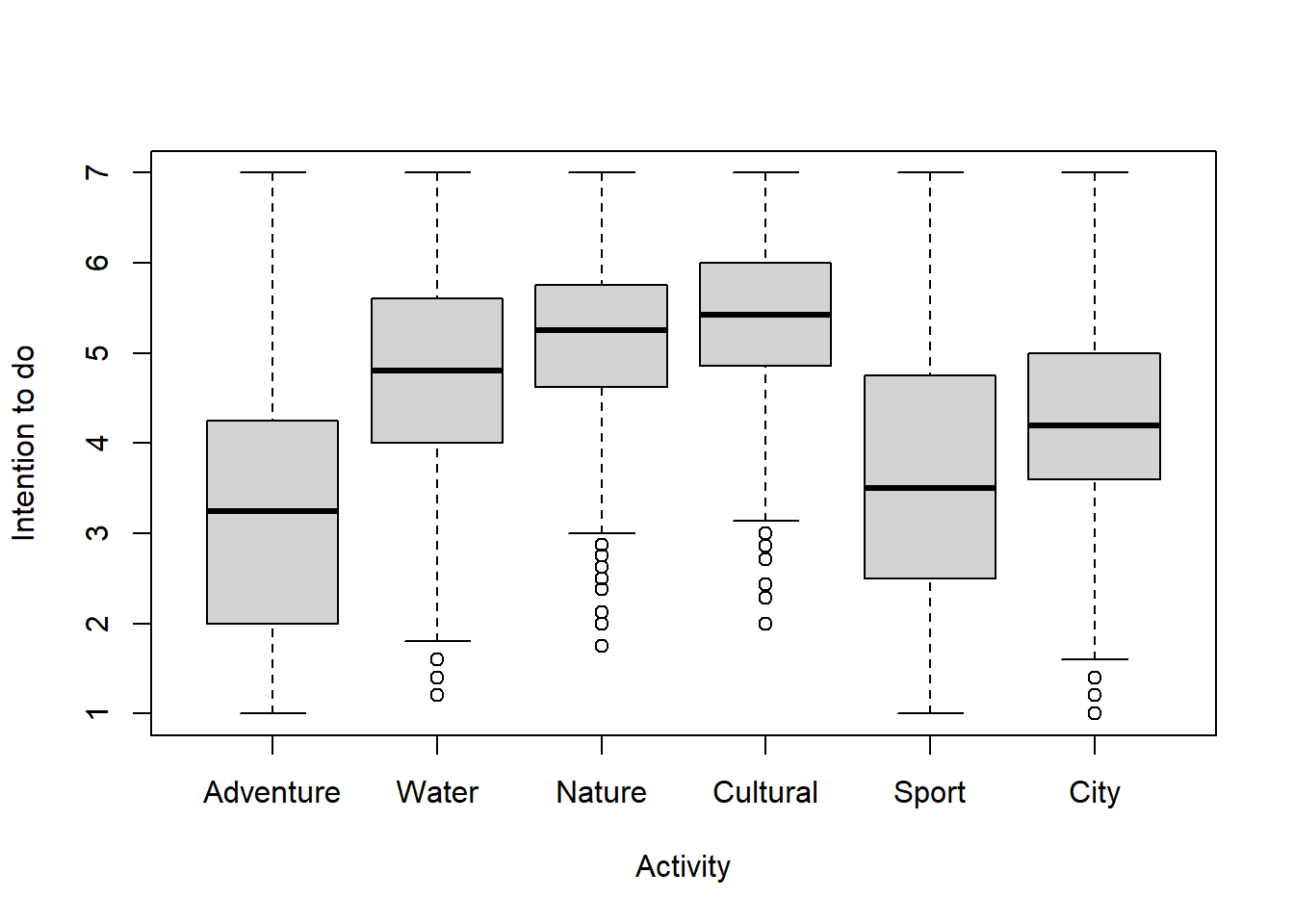

Nature and Cultural activities have highest median ratings and the smallest spread (variation) in ratings.

Adventure and Sport activities have the lowest median ratings and the largest spread (variation) in ratings.

Create and interpret box plots for the Australian and German data.

2d. Difference in Means (paired)

Nature and Cultural activities appear to be the most popular, at least in terms of intentions to engage in. As you have seen in the previous tasks, Cultural activities have a slightly higher mean and median rating. Test if this difference is significant using a paired t.test() for a single comparison between means.

Why have we carried out a paired t.test?

Interpret the 95% confidence interval and corresponding p-value for the t.test.

Code

#first test if variances are equal
var.test(before_japan$Nature,before_japan$Cultural, alternative = "two.sided") 

#significant evidence against null hypothesis that variances are equal, use var.equal=F in t test
t.test(before_japan$Nature,before_japan$Cultural,var.equal = T,paired=T)

Code

#first test if variances are equal
var.test(before_japan$Nature,before_japan$Cultural, alternative = "two.sided")


    F test to compare two variances

data:  before_japan$Nature and before_japan$Cultural
F = 0.91679, num df = 983, denom df = 986, p-value = 0.1731
alternative hypothesis: true ratio of variances is not equal to 1
95 percent confidence interval:
 0.8090637 1.0388656
sample estimates:
ratio of variances 
          0.916787

Code

#no significant evidence against null hypothesis that variances are equal, use var.equal=T in t test
t.test(before_japan$Nature,before_japan$Cultural,var.equal = T,paired=T)


    Paired t-test

data:  before_japan$Nature and before_japan$Cultural
t = -11.271, df = 961, p-value < 2.2e-16
alternative hypothesis: true mean difference is not equal to 0
95 percent confidence interval:
 -0.3458347 -0.2432654
sample estimates:
mean difference 
       -0.29455

Paired t-tests are used when the data for both groups is collected from the same participants - either at different time points or in different contexts. In our case, the same tourists have provided intention ratings for nature related and cultural activities.

The p-value is much smaller than 0.05, indicating highly significant evidence against the null hypothesis that the mean difference in ratings is equal to 0. Therefore, we can reject the null in favour of the alternative hypothesis - a true mean difference in pre-trip ratings of Nature and Cultural activities. We can be 95% confident that the true mean ratings for Nature activities are between 0.2432654 and 0.3458347 lower than Cultural.

Based on the box plots constructed in Task 2c., choose some activities to compare using t.test() for the German and Australian data.

3. Histograms, Proportion Tables, Difference in Proportions

We will investigate the demographic characteristics of Japanese tourists intending to visit New Zealand.

3a. Histogram

Construct an appropriately labelled histogram of the Age of potential Japanese tourists to New Zealand. Select and set colours for both the bars and their outlines.

What does this histogram tell you about the age distribution?

Code

#breaks=50 to show more distribution detail
hist(before_japan$Age,breaks=50,xlab="Years", col="skyblue",border="red3",
    main="Age distribution of Japanese tourists to New Zealand")

Code

#breaks=50 to show more distribution detail
hist(before_japan$Age,breaks=50,xlab="Years",col="skyblue",border="red3",
    main="Age distribution of Japanese tourists to New Zealand")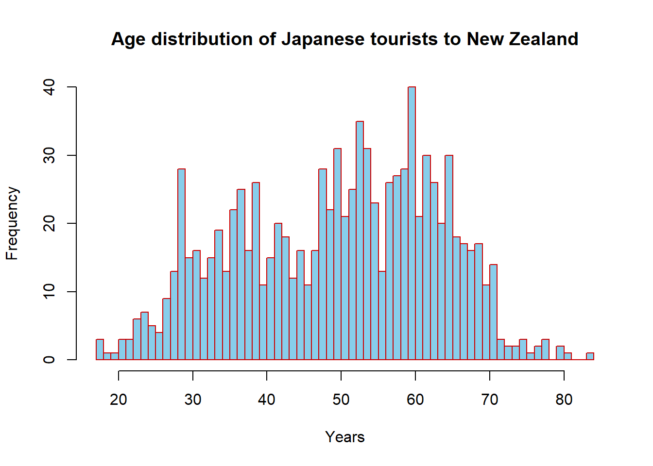

The ages of potential Japanese tourists to New Zealand are fairly evenly distributed from 30 to 70 years old (with few below 30 or above 70 years included in the survey), with a slightly higher frequency in the 50-70 range compared to the 30-50 range.

Construct histograms of the ages of Australian and German tourists. How do these distributions compare to the Japanese tourists?

Important Information

3b. Histogram

Construct an appropriately labelled histogram of the intended LengthStay of potential Japanese tourists to New Zealand. This has a very long tail (positive skew), so try setting some different xlim=c(,) values in order to get a more detailed picture of the most common intended stay lengths.

Interpret the distribution of intended stay length.

Code

#breaks=200 for detail, xlim=c(0,30) to focus on most common short stays
hist(before_japan$LengthStay,breaks=200,xlab="Days",
     main="Length of stay of Japanese tourists to New Zealand",xlim=c(0,30))

Code

#breaks=200 for detail, xlim=c(0,30) to focus on most common short stays
hist(before_japan$LengthStay,breaks=200,xlab="Days",
     main="Length of stay of Japanese tourists to New Zealand",xlim=c(0,30))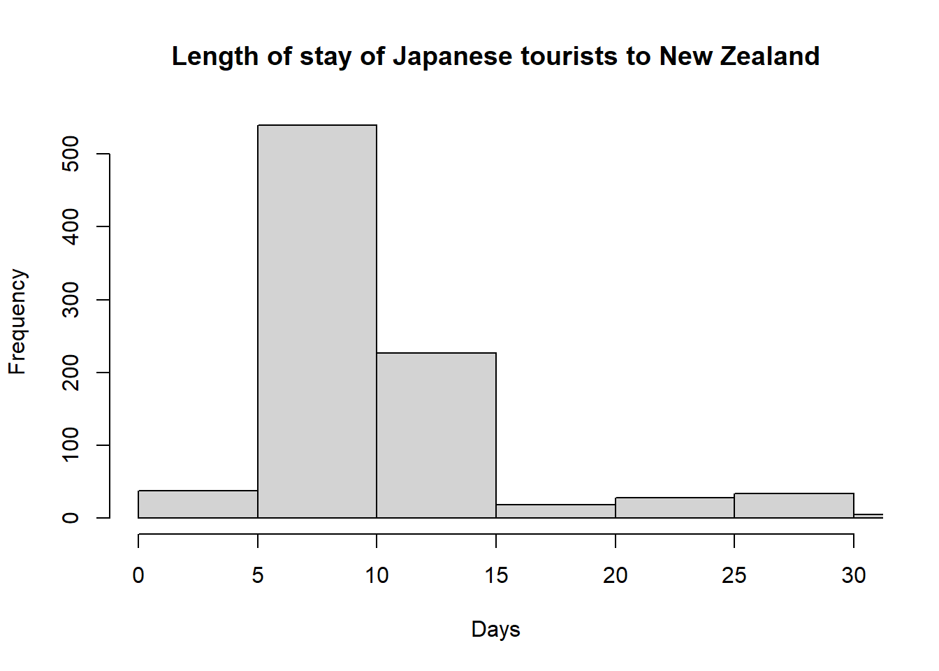

The vast majority of planned stay lengths are between 5 and 15 days, however without the xlim restriction we see that a few Japanese tourists plan to stay for a year or even longer.

Repeat for the intended stay length of German and Australian tourists. Compare all three distributions.

Important Information

3c. Proportion Table

There is data for several factor (categorical) demographic variables, TravelStyle, Transport, Accom, Gender and Income. Check the proportion of potential tourists in each category of these using the table() and prop.table() functions, as you have done in previous lessons.

For each factor variable, find the categories with the smallest and largest proportion of potential Japanese tourists. Consider if there is a lot of variation between categories, or a more even distribution of tourists?

Code

#table() first to calculate counts, prop.table() to convert these to proportions
prop.table(table(before_japan$TravelStyle))
prop.table(table(before_japan$Transport))
prop.table(table(before_japan$Accom))
prop.table(table(before_japan$Gender))
prop.table(table(before_japan$Income))

Code

#table() first to calculate counts, prop.table() to convert these to proportions
prop.table(table(before_japan$TravelStyle))


       Free          NA     Package SemiPackage 
  0.3150147   0.1118744   0.2325810   0.3405299

Code

prop.table(table(before_japan$Transport))


        Bus   Campervan         Car        Comb          NA       Other 
0.280667321 0.175662414 0.002944063 0.192345437 0.185475957 0.004906771 
      Plane       Train 
0.046123651 0.111874387

Code

prop.table(table(before_japan$Accom))


Backpackers         BnB      Camper        Comb       Hotel       Motel 
0.013738960 0.098135427 0.003925417 0.056918548 0.595682041 0.051030422 
         NA       Other 
0.156035329 0.024533857

Code

prop.table(table(before_japan$Gender))


        1         2 
0.6344196 0.3655804

Code

prop.table(table(before_japan$Income))


         1          2          3          4          5          6          7 
0.04766949 0.07627119 0.07627119 0.05826271 0.07203390 0.06779661 0.08474576 
         8          9         10         11         12 
0.09851695 0.25529661 0.09110169 0.03283898 0.03919492

Semi-package tours are the most popular tour style choice for potential Japanese tourists to NZ, with full package being the least popular.

Nearly a third of the potential tourists surveyed intended to travel by bus, and almost none intended to drive while here.

Over half of Japanese tourists planned to stay in a hotel on their trip and staying in a campervan was the least appealing option.

The amount of male potential tourists was almost double the amount of female.

There was reasonable spread in the income distributions of prospective Japanese tourists, however the largest category accounting for a quarter of those surveyed was 1000 to 1500.

Compare the travel choices and demographic characteristics of German and Australian tourists.

Important Information

3d. Difference in Proportions

The difference in Gender proportion of tourists may be worth investigating. Check if this is significant using prop.test().

Interpret the 95% confidence interval and corresponding p-value.

Code

#First argument is the number of successes (in this case having gender=1, being male)
#second argument is number of trials (total gender observations)
#note the use of length to sum the counts
prop.test(length(which(before_japan$Gender==1)),n=length(before_japan$Gender))

Code

#First argument is the number of successes (in this case having gender=1, being male)
#second argument is number of trials (total gender observations)
#note the use of length to sum the counts
prop.test(c(length(which(before_japan$Gender==1)),length(which(before_japan$Gender==2))),n=c(length(before_japan$Gender),length(before_japan$Gender)))


    2-sample test for equality of proportions with continuity correction

data:  c(length(which(before_japan$Gender == 1)), length(which(before_japan$Gender == 2))) out of c(length(before_japan$Gender), length(before_japan$Gender))
X-squared = 135.94, df = 1, p-value < 2.2e-16
alternative hypothesis: two.sided
95 percent confidence interval:
 0.2161926 0.3019625
sample estimates:
   prop 1    prop 2 
0.6113837 0.3523062

The p-value is much smaller than 0.05, indicating highly significant evidence against the null hypothesis that the difference in proportion of male and female prospective Japanese tourists is equal to 0. Therefore, we can reject the null in favour of the alternative hypothesis - a true difference in proportion of male and female tourists. We can be 95% confident that the true proportion of male tourists is between 0.2252230 and 0.3124552 higher than the true proportion of female tourists.

Identify some interesting categories for comparison from the German and Australian data, then check for significant differences using prop.test()

Important Information

4. Function Writing, Proportion Summary Table

Now we will examine data from Japanese tourists who have already visited New Zealand, using the after_japan data frame.

Create a table that contains, for all activities, the percentage of tourists who engaged in it and the percentage that considered it a highlight.

Use the knitr package to present this table in an attractive format.

What patterns can you see in terms of activities that are engaged in by a high percentage of Japanese tourists, and activities that are considered highlights by a high percentage of Japanese tourists?

To calculate the percentage of tourists who engaged in each activity we will need to create a function. This is a good opportunity to practice writing a function in R.

You can also reveal the code to see how to do this.

Code

#function has two arguments, the observations (x) and the threshold (thres). 
#thres defaults to 2, as this represents engaging in an activity at least once
propFun<-function(,){
  temp<-  #remove NAs and create new variable temp
    #find proportion above thres (tourists who engaged in activity at least once), 
    #out of total observations (tourists who responded)
  propX<-length(which( ))/length( ) 
  return( ) #return proportion
}

Code

#function has two arguments, the observations (x) and the threshold (thres). 
#thres defaults to 2, as this represents engaging in an activity at least once
propFun<-function(x,thres=2){
  temp<-x[!is.na(x)] #remove NAs
  #find proportion above thres (tourists who engaged in activity at least once), 
  #out of total observations (tourists who responded)
  propX<-length(which(temp>=thres))/length(temp) 
  return(propX) #return proportion
}

Using the inbuilt mean() function on the highlight binary variables will calculate the proportion of tourists who considered each activity a highlight, as it will add up all entries (1 or 0) and divide this by the total number of observations.

We can now calculate the relevant proportions using the apply() function.

Code

#calculate proportion of tourists who engaged in each activity using apply() and your custom function
#every second variable, from column 2 to 66, is the frequency of activity engagement
freq<-apply(after_japan[seq(from=35,to=99,by=2)],MARGIN = 2,FUN=propFun)

#calculate proportion of tourists who considered each activity a highlight using apply() and mean
#every second variable, from column 3 to 67, is the binary highlight rating
high<-apply(after_japan[seq(from=36, to=100,by=2)],MARGIN=2,FUN=mean,na.rm=T)

Using mean() to determine highlight percentage does not take into account whether tourists actually engaged in the particular activity, as tourists who did not engage will automatically not be able to consider it a highlight.

The code to calculate highlight percentage given engagement is available below in the next hidden chunk, it is slightly more complex involving a for() loop and some unfamiliar functions. This can be skipped, but if you are interested, you can calculate these new percentages and compare them with those generated by simply taking the mean.

Code

cols<-seq(36,100,by=2)
highprop<-c()
for(i in cols){
  engaged<-c(after_japan[which(after_japan[,i-1]>=2),i])
  prop<- eval(parse(text=paste("engaged$`",colnames(after_japan[,i]),"`",sep="")))
  highprop<- c(highprop,mean(prop,na.rm=TRUE))
   
}

To view the results, group the percentage of tourists who engaged in each activity and the percentage that considered it a highlight together using cbind(), and subset this object to display them in order of decreasing frequency or highlight consideration.

Code

#multiply by 100 to convert proportion to percentage
#order by decreasing percentage engaged
f<-cbind(PercentDoneBy = freq*100,PercentConsideredHighlight = high*100) [order(-freq),]

#nice table
kable(f,digits=3)

Code

#multiply by 100 to convert proportion to percentage
#order by decreasing percentage considered highlight
h<-cbind(PercentDoneBy = freq*100,PercentConsideredHighlight = high*100) [order(-high),]

#nice table
kable(h,digits=3)

Comparison with highlight percentages when incorporating engagement is available below.

Code

#multiply by 100 to convert proportion to percentage
#order by decreasing percentage considered highlight
hp<-cbind(PercentDoneBy = freq*100,Highlight = high*100,HighlightGivenEngagement=highprop*100) [order(-highprop),]

#nice table
kable(hp,digits=3)

To calculate the percentage of tourists who engaged in each activity we will need to create a function. This is a good opportunity to practice writing a function in R.

Code

#function has two arguments, the observations (x) and the threshold (thres). 
#thres defaults to 2, as this represents engaging in an activity at least once
propFun<-function(,){
  temp<-  #remove NAs and create new variable temp
    #find proportion above thres (tourists who engaged in activity at least once), 
    #out of total observations (tourists who responded)
  propX<-length(which( ))/length( ) 
  return( ) #return proportion
}

Code

#function has two arguments, the observations (x) and the threshold (thres). 
#thres defaults to 2, as this represents engaging in an activity at least once
propFun<-function(x,thres=2){
  temp<-x[!is.na(x)] #remove NAs
  #find proportion above thres (tourists who engaged in activity at least once), 
  #out of total observations (tourists who responded)
  propX<-length(which(temp>=thres))/length(temp) 
  return(propX) #return proportion
}

We can now calculate the relevant proportions using the apply() function.

Code

#calculate proportion of tourists who engaged in each activity using apply() and your custom function
#every second variable, from column 2 to 66, is the frequency of activity engagement
freq<-apply(after_japan[seq(from=35,to=99,by=2)],MARGIN = 2,FUN=propFun)

#calculate proportion of tourists who considered each activity a highlight using apply() and mean
#every second variable, from column 3 to 67, is the binary highlight rating
high<-apply(after_japan[seq(from=36, to=100,by=2)],MARGIN=2,FUN=mean,na.rm=T)

Code

cols<-seq(36,100,by=2)
highprop<-c()
for(i in cols){
  engaged<-c(after_japan[which(after_japan[,i-1]>=2),i])
  prop<- eval(parse(text=paste("engaged$`",colnames(after_japan[,i]),"`",sep="")))
  highprop<- c(highprop,mean(prop,na.rm=TRUE))
   
}

Code

#multiply by 100 to convert proportion to percentage
#order by decreasing percentage engaged
f<-cbind(PercentDoneBy = freq*100,PercentConsideredHighlight = high*100) [order(-freq),]

#nice table
kable(f,digits=3)

	PercentDoneBy	PercentConsideredHighlight
aShop	96.729	6.697
aShortWalk	96.659	17.249
aCuisine	86.730	7.075
aLocals	81.995	15.677
aMuseum/Gallery	81.146	9.198
aBotanicGarden	68.116	7.177
aSightSeeTour	67.070	11.722
aBoatTour	66.351	13.176
aHike/Tramp	64.010	17.021
aMarae	61.814	6.383
aCulturalPerform	60.291	11.058
aGlacier	48.804	14.421
aHistoric	45.012	2.651
aEveningEntertainment	38.107	2.871
aSunbathe	37.192	2.676
aMarine	35.507	4.327
aBirdWatch	34.217	2.387
aScenicFlight	33.412	11.475
aSpecialEvent	29.426	4.048
aJetBoat	28.271	8.879
aSwim	24.408	1.425
aFarmstay	19.093	7.126
aShows	18.005	1.695
aGolf	15.534	2.663
aRaft	14.908	6.422
aCasino	12.619	1.446
aKayak/Canoe	11.005	2.387
aHunt/Fish	9.135	1.699
aSki	7.857	3.865
aWinterSport	7.674	1.435
aDolphinSwim	5.213	3.066
aBungy	4.941	5.841
aParachute	3.783	2.594

Code

#multiply by 100 to convert proportion to percentage
#order by decreasing percentage considered highlight
h<-cbind(PercentDoneBy = freq*100,PercentConsideredHighlight = high*100) [order(-high),]

#nice table
kable(h,digits=3)

	PercentDoneBy	PercentConsideredHighlight
aShortWalk	96.659	17.249
aHike/Tramp	64.010	17.021
aLocals	81.995	15.677
aGlacier	48.804	14.421
aBoatTour	66.351	13.176
aSightSeeTour	67.070	11.722
aScenicFlight	33.412	11.475
aCulturalPerform	60.291	11.058
aMuseum/Gallery	81.146	9.198
aJetBoat	28.271	8.879
aBotanicGarden	68.116	7.177
aFarmstay	19.093	7.126
aCuisine	86.730	7.075
aShop	96.729	6.697
aRaft	14.908	6.422
aMarae	61.814	6.383
aBungy	4.941	5.841
aMarine	35.507	4.327
aSpecialEvent	29.426	4.048
aSki	7.857	3.865
aDolphinSwim	5.213	3.066
aEveningEntertainment	38.107	2.871
aSunbathe	37.192	2.676
aGolf	15.534	2.663
aHistoric	45.012	2.651
aParachute	3.783	2.594
aKayak/Canoe	11.005	2.387
aBirdWatch	34.217	2.387
aHunt/Fish	9.135	1.699
aShows	18.005	1.695
aCasino	12.619	1.446
aWinterSport	7.674	1.435
aSwim	24.408	1.425

Relaxed and cultural activities are the most engaged in by Japanese tourists in New Zealand - more than 80% of those surveyed participated in shopping, short walks, meeting locals and visiting museums/galleries. Adventure based activities such as skiing, winter sports, parachute and bungy jumping were the least popular. They were engaged in by less than 10% of Japanese tourists.

Without taking into account initial engagement, nature based activities (short walk, hike/tramp, glacier, boat and sight seeing tours) were the most commonly considered trip highlights for Japanese tourists, possibly due to New Zealand’s unique scenery.

Comparison with highlight percentages when incorporating engagement is available below.

Code

#multiply by 100 to convert proportion to percentage
#order by decreasing percentage considered highlight
hp<-cbind(PercentDoneBy = freq*100,Highlight = high*100,HighlightGivenEngagement=highprop*100) [order(-highprop),]

#nice table
kable(hp,digits=3)

	PercentDoneBy	Highlight	HighlightGivenEngagement
aBungy	4.941	5.841	52.381
aSki	7.857	3.865	39.394
aParachute	3.783	2.594	37.500
aRaft	14.908	6.422	33.846
aFarmstay	19.093	7.126	33.750
aScenicFlight	33.412	11.475	31.690
aJetBoat	28.271	8.879	29.752
aGlacier	48.804	14.421	26.961
aHike/Tramp	64.010	17.021	23.019
aDolphinSwim	5.213	3.066	22.727
aBoatTour	66.351	13.176	18.929
aKayak/Canoe	11.005	2.387	17.391
aLocals	81.995	15.677	16.914
aCulturalPerform	60.291	11.058	16.867
aHunt/Fish	9.135	1.699	15.789
aShortWalk	96.659	17.249	15.556
aSightSeeTour	67.070	11.722	15.523
aGolf	15.534	2.663	14.062
aWinterSport	7.674	1.435	12.500
aSpecialEvent	29.426	4.048	11.382
aCasino	12.619	1.446	11.321
aMarine	35.507	4.327	10.204
aMuseum/Gallery	81.146	9.198	9.735
aBotanicGarden	68.116	7.177	9.220
aMarae	61.814	6.383	8.494
aCuisine	86.730	7.075	7.397
aShop	96.729	6.697	5.797
aShows	18.005	1.695	5.405
aSwim	24.408	1.425	4.902
aEveningEntertainment	38.107	2.871	4.459
aBirdWatch	34.217	2.387	4.225
aSunbathe	37.192	2.676	3.974
aHistoric	45.012	2.651	3.243

After taking into account initial engagement, adventure based activities (bungy jump, skiing, parachuting, rafting) are considered highlights by the largest percentage of tourists who took part in them. Farm stays were trip highlights for a third of tourists who visited them. As these activities were not engaged in as frequently, a low total percentage of Japanese tourists reported them as highlights. However, people who did engage with them typically enjoyed them.

Repeat this exercise for the Australian and German tourist data.

Important Information

5. New Variables, Box Plots

5a. New Variables

Modify code from Task 2a. to group the frequency of engagement variables (beginning with a) into broader categories by calculating an average weighting across them for each respondent. Use the same groupings as for the before_japan data frame Adventure, Water, Nature. Cultural, Sport and City.

Code

#four groupings that we will consider, creating new variables to represent these
#sum individual ratings and divide by number of original variables to find mean

after_japan$Adventure=(after_japan$aRaft+after_japan$aJetBoat+after_japan$aBungy+
                      after_japan$aParachute)/4
after_japan$Water=(after_japan$aDolphinSwim+after_japan$aSwim+after_japan$aBoatTour+
                    after_japan$aMarine+after_japan$aSunbathe)/5
after_japan$Nature=(after_japan$aShortWalk+after_japan$`aHike/Tramp`+
  after_japan$`aHunt/Fish`+after_japan$aScenicFlight+after_japan$aBotanicGarden+
    after_japan$aBirdWatch+after_japan$aGlacier+after_japan$aFarmstay)/8
after_japan$Cultural=(after_japan$`aMuseum/Gallery`+after_japan$aCulturalPerform+
    after_japan$aMarae+after_japan$aHistoric+after_japan$aLocals+
      after_japan$aSightSeeTour+after_japan$aCuisine)/7

after_japan$Sport=(after_japan$`aKayak/Canoe`+after_japan$aWinterSport+
                     after_japan$aSki+after_japan$aGolf)/4
after_japan$City=(after_japan$aShop+after_japan$aEveningEntertainment+
    after_japan$aSpecialEvent+after_japan$aShows+after_japan$aCasino)/5

Code

#four groupings that we will consider, creating new variables to represent these
#sum individual ratings and divide by number of original variables to find mean

after_japan$Adventure=(after_japan$aRaft+after_japan$aJetBoat+after_japan$aBungy+
                      after_japan$aParachute)/4
after_japan$Water=(after_japan$aDolphinSwim+after_japan$aSwim+after_japan$aBoatTour+
                    after_japan$aMarine+after_japan$aSunbathe)/5
after_japan$Nature=(after_japan$aShortWalk+after_japan$`aHike/Tramp`+
  after_japan$`aHunt/Fish`+after_japan$aScenicFlight+after_japan$aBotanicGarden+
    after_japan$aBirdWatch+after_japan$aGlacier+after_japan$aFarmstay)/8
after_japan$Cultural=(after_japan$`aMuseum/Gallery`+after_japan$aCulturalPerform+
    after_japan$aMarae+after_japan$aHistoric+after_japan$aLocals+
      after_japan$aSightSeeTour+after_japan$aCuisine)/7

after_japan$Sport=(after_japan$`aKayak/Canoe`+after_japan$aWinterSport+
                     after_japan$aSki+after_japan$aGolf)/4
after_japan$City=(after_japan$aShop+after_japan$aEveningEntertainment+
    after_japan$aSpecialEvent+after_japan$aShows+after_japan$aCasino)/5

Repeat for the German and Australian data if you wish to continue the extension into the next part of the lesson.

Important Information

5b. Box Plots

Create box plots of the frequencies of engagement in the summary categories Adventure, Water, Nature. Cultural, Sport and City.

Plot these beside the box plots of intentions to engage, with boxes coloured to correspond to the different summary categories.

Based on these results, how do the actual frequencies of engagement compare to the pre-trip intentions to engage?

Code

boxplot(after_japan$Adventure,after_japan$Water,after_japan$Nature,after_japan$Cultural,after_japan$Sport,after_japan$City,names=c("Adventure","Water","Nature","Cultural","Sport","City"),ylab="Frequency of Engagement",xlab="Activity",col=c("orangered1","paleturquoise2","chartreuse3","red3","darkorchid","yellow2"))

Code

par(mfrow=c(1,2)) #arrange plots beside each other (1 row, 2 columns) for more direct comparison
boxplot(after_japan$Adventure,after_japan$Water,after_japan$Nature,after_japan$Cultural,after_japan$Sport,after_japan$City,names=c("Adventure","Water","Nature","Cultural","Sport","City"),ylab="Frequency of Engagement",xlab="Activity",col=c("orangered1","paleturquoise2","chartreuse3","red3","darkorchid","yellow2"))

boxplot(before_japan$Adventure,before_japan$Water,before_japan$Nature,before_japan$Cultural,before_japan$Sport,before_japan$City,names=c("Adventure","Water","Nature","Cultural","Sport","City"),ylab="Intention to do",xlab="Activity",col=c("orangered1","paleturquoise2","chartreuse3","red3","darkorchid","yellow2"))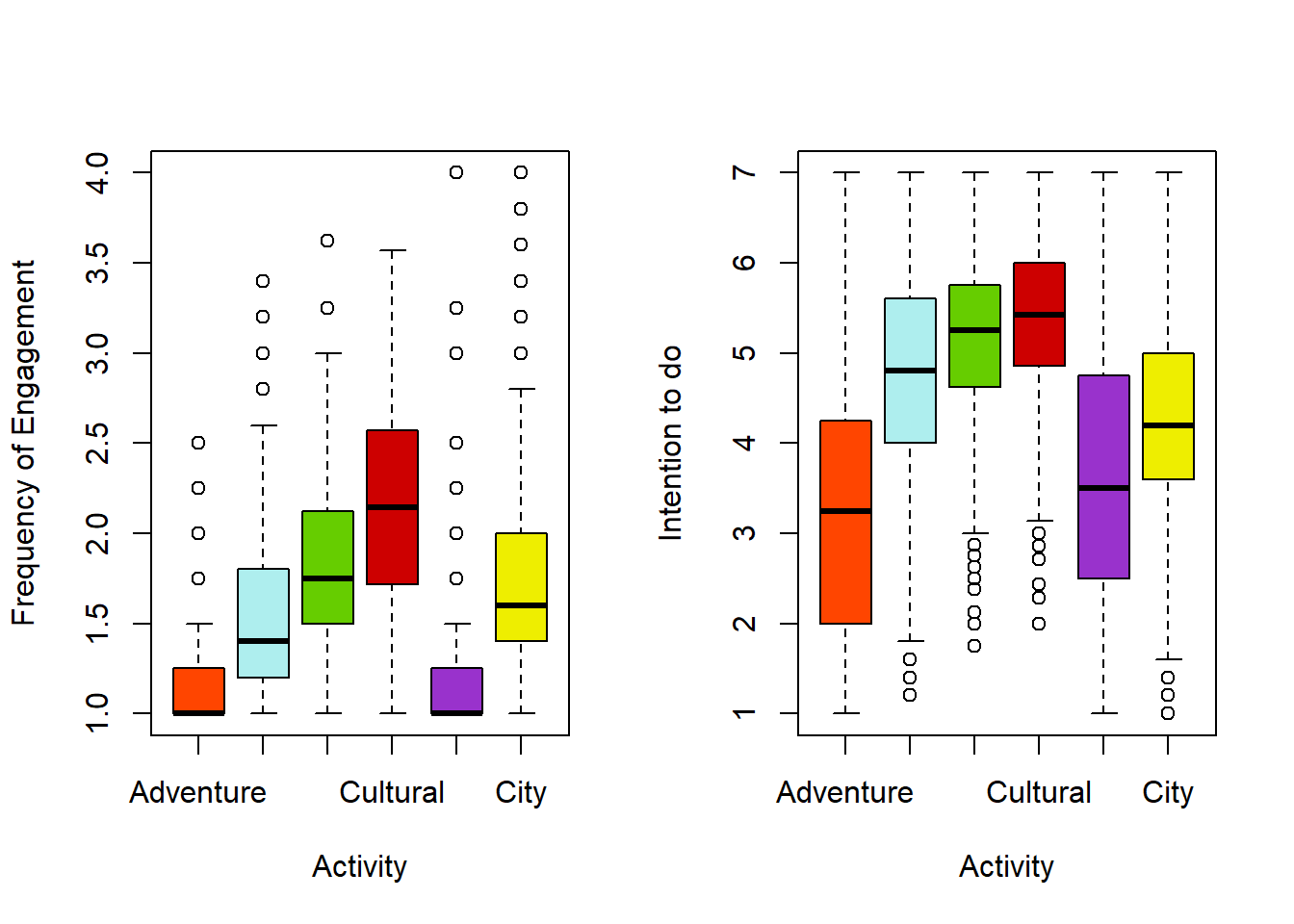

Cultural activities were the most engaged in by Japanese tourists, Sport and Adventure activities were engaged in the least. This matches the findings regarding pre-trip intentions (there is some overlap in respondents, but also considerable differences in the sample). City activities tended to be actually engaged in during a New Zealand trip with greater frequency than was planned by those surveyed before their trips. This may be because tourists typically arrive in a city (either by plane or cruise) and are most likely to base themselves in one to access the most activities with the least travel, so even if spending time in a city is not something they are excited about pre-trip it is where they end up for practical reasons.

Create analogous box plots for the German and Australian data.

6. Data Reformatting, Tables, Line Plots, For Loops

6a. Data Reformatting

Convert the highlight ratings gathered after engagement in each activity into long format, according to their assigned summary category (Adventure, Water, Nature, Cultural, Sport, City).

Data in long format has a row for each observation (activity) and a column for each variable (rating).

Code

library(tidyr)

#adventure category, specify columns that contain binary highlight ratings for the relevant activities (rafting, bungy, parachute, jet boat)
japanLongA<-gather(data=after_japan,key="hAdventure",value="Rating",c(36,38,40,44))

Modify this code to repeat for the remaining categories.

Code

library(tidyr)

#adventure category, specify columns that contain binary highlight ratings for the relevant activities (rafting, bungy, parachute, jet boat)
japanLongA<-gather(data=after_japan,key="hAdventure",value="Rating",c(36,38,40,44))

#water category, specify columns that contain binary highlight ratings for the relevant activities
japanLongW<-gather(data=after_japan,key="hWater",value="Rating",c(42,46,76,92,100))

#nature category, specify columns that contain binary highlight ratings for the relevant activities
japanLongN<-gather(data=after_japan,key="hNature",value="Rating",c(58,60,64,74,84,86,90,98))

#cultural category, specify columns that contain binary highlight ratings for the relevant activities
japanLongC<-gather(data=after_japan,key="hCultural",value="Rating",c(50,52,62,70,78,80,94))

#sport category, specify columns that contain binary highlight ratings for the relevant activities
japanLongS<-gather(data=after_japan,key="hSport",value="Rating",c(48,66,68,96))

#city category, specify columns that contain binary highlight ratings for the relevant activities
japanLongY<-gather(data=after_japan,key="hCity",value="Rating",c(54,56,72,82,88))

This can be repeated for the Australian and German tourist data.

Important Information

6b. Count Tables

Create a table that summarises the consideration of the Adventure activities as highlights by gender for Japanese tourists. Make sure to include row and column totals, and informative dimension names.

Use the knitr package to present this table in an attractive format.

Are there any major differences in which activities are considered highlights by male and female respondents?

Code

#subset to include only ratings equal to 1 (highlights)
japan<-japanLongA[japanLongA$Rating==1,]

#table of adventure activities considered highlights by gender, label rows and columns using dnn
a<-addmargins(table(japan$Gender,japan$hAdventure,dnn=c("Gender","Adventure")))
kable(a)

Repeat for the other summary categories, and investigate the changes between some different demographic variables.

Code

#subset to include only ratings equal to 1 (highlights)
japanA<-japanLongA[japanLongA$Rating==1,]

#table of adventure activities considered highlights by gender, label rows and columns using dnn
a<-addmargins(table(japanA$Gender,japanA$hAdventure,dnn=c("Gender","Adventure")))
kable(a)

	hBungy	hJetBoat	hParachute	hRaft	Sum
1	18	17	4	10	49
2	5	18	6	14	43
Sum	23	35	10	24	92

Code

japanW<-japanLongW[japanLongW$Rating==1,]
w<-addmargins(table(japanW$Gender,japanW$hWater,dnn=c("Gender","Water")))
kable(w)

	hBoatTour	hDolphinSwim	hMarine	hSunbathe	hSwim	Sum
1	25	3	11	3	3	45
2	29	9	6	8	3	55
Sum	54	12	17	11	6	100

Code

japanN<-japanLongN[japanLongN$Rating==1,]
n<-addmargins(table(japanN$Education,japanN$hNature,dnn=c("Education","Nature")))
kable(n)

	hBirdWatch	hBotanicGarden	hFarmstay	hGlacier	hHike/Tramp	hHunt/Fish	hScenicFlight	hShortWalk	Sum
1	2	5	3	8	10	1	6	18	53
2	2	5	10	9	18	3	6	16	69
3	5	16	12	35	34	3	29	32	166
4	1	4	4	7	5	0	3	6	30
Sum	10	30	29	59	67	7	44	72	318

Code

japanC<-japanLongC[japanLongC$Rating==1,]
c<-addmargins(table(japanC$Transport,japanC$hCultural,dnn=c("Transport","Cultural")))
kable(c)

	hCuisine	hCulturalPerform	hHistoric	hLocals	hMarae	hMuseum/Gallery	hSightSeeTour	Sum
Bus	6	22	3	13	10	11	14	79
Campervan	2	1	2	9	1	3	5	23
Car	0	1	0	1	0	0	0	2
Comb	8	10	3	15	5	13	10	64
NA	4	5	1	10	6	6	9	41
Other	5	2	0	10	2	2	4	25
Plane	5	4	2	7	3	4	7	32
Train	0	1	0	1	0	0	0	2
Sum	30	46	11	66	27	39	49	268

Code

japanS<-japanLongS[japanLongS$Rating==1,]
s<-addmargins(table(japanS$TravelStyle,japanS$hSport,dnn=c("Travel Style","Sport")))
kable(s)

	hGolf	hKayak/Canoe	hSki	hWinterSport	Sum
Free	5	7	8	2	22
NA	2	3	5	3	13
Package	2	0	2	1	5
SemiPackage	2	0	1	0	3
Sum	11	10	16	6	43

Code

japanY<-japanLongY[japanLongY$Rating==1,]
y<-addmargins(table(japanY$Gender,japanY$hCity,dnn=c("Gender","City")))
kable(y)

	hCasino	hEveningEntertainment	hShop	hShows	hSpecialEvent	Sum
1	2	3	12	0	8	25
2	4	8	15	6	8	41
Sum	6	11	27	6	16	66

Repeat this exercise for the Australian and German tourist data.

Important Information

6c. Proportion Tables, Line Plots

Convert the contingency tables in 6b. to proportion tables.

Format these proportion tables as matrices, then create line plots of the proportion considering each activity a highlight. These plots should have a separate line for each level of the demographic variable of interest.

Code

#proportion table from table of counts, rows (Gender) sum to 1
pAdventure<-prop.table(table(japanA$Gender,japanA$hAdventure,dnn=c("Gender","Adventure")),margin=1)

kable(pAdventure,digits=3)

Code

#convert proportion table to matrix format for plotting
mAdventure<-matrix(pAdventure,nrow=2,ncol=4)

#construct base plot with line for males, remove axis to allow relabelling
plot(mAdventure[1,],ylim=c(0,1),ylab="Proportion considering highlight",type="o",xaxt="n",xlab="Activity",col="red",pch=20)

#add line for females
points(mAdventure[2,],type="o",col="green",pch=20)

#add x axis with appropriate labels
axis(1,at=c(1,2,3,4),labels=c("Bungy","Jet Boat","Parachute","Raft"))

#legend to distinguish lines
legend("topright",legend=c("Male","Female"),pch=20,col=c("red","green"))

Code

#proportion table from table of counts, rows (Gender) sum to 1
pAdventure<-prop.table(table(japanA$Gender,japanA$hAdventure,dnn=c("Gender","Adventure")),margin=1)

kable(pAdventure,digits=3)

hBungy	hJetBoat	hParachute	hRaft
0.367	0.347	0.082	0.204
0.116	0.419	0.140	0.326

Code

#convert proportion table to matrix format for plotting
mAdventure<-matrix(pAdventure,nrow=2,ncol=4)

#construct base plot with line for males, remove axis to allow relabelling
plot(mAdventure[1,],ylim=c(0,1),ylab="Proportion considering highlight",type="o",xaxt="n",xlab="Activity",col="red",pch=20)

#add line for females
points(mAdventure[2,],type="o",col="green",pch=20)

#add x axis with appropriate labels
axis(1,at=c(1,2,3,4),labels=c("Bungy","Jet Boat","Parachute","Raft"))

#legend to distinguish lines
legend("topright",legend=c("Male","Female"),pch=20,col=c("red","green"))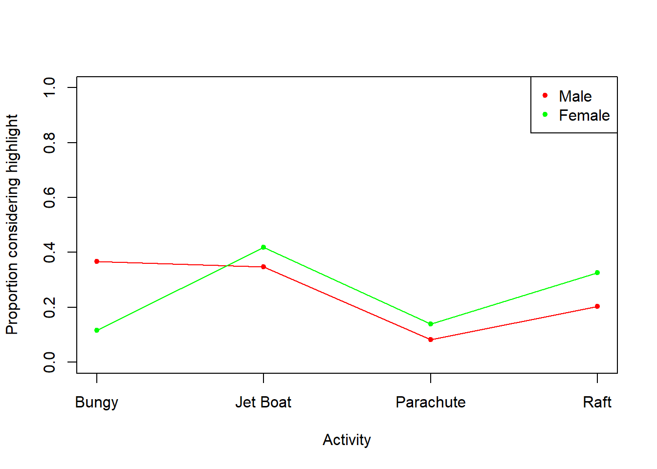

Similar proportions of male and female Japanese tourists considered jet boat, parachute, and rafting trip highlights. However, there is a notably greater proportion of males who considered bungy the highlight of their stay. This suggests bungy jump advertising may be better targeted towards males than females.

Code

#proportion table from table of counts, rows (Gender) sum to 1
pSport<-prop.table(table(japanS$TravelStyle,japanS$hSport,dnn=c("Travel Style","Sport")),margin=1)

kable(pSport,digits=3)

	hGolf	hKayak/Canoe	hSki	hWinterSport
Free	0.227	0.318	0.364	0.091
NA	0.154	0.231	0.385	0.231
Package	0.400	0.000	0.400	0.200
SemiPackage	0.667	0.000	0.333	0.000

Code

#convert proportion table to matrix format for plotting
mSport<-matrix(pSport,nrow=4,ncol=4)

#construct base plot with line for free travel style, remove axis to allow relabelling
plot(mSport[1,],ylim=c(0,1),ylab="Proportion considering highlight",type="o",xaxt="n",xlab="Activity",col="red",pch=20)

#add lines for NA, package, semi package travel styles
points(mSport[2,],type="o",col="green",pch=20)

points(mSport[3,],type="o",col="blue",pch=20)

points(mSport[4,],type="o",col="orange",pch=20)

#add x axis with appropriate labels
axis(1,at=c(1,2,3,4),labels=c("Golf","Kayak/Canoe","Ski","Winter Sport"))

#legend to distinguish lines
legend("topright",legend=c("Free","Package","Semi Package","NA"),pch=20,col=c("red","blue","orange","green"))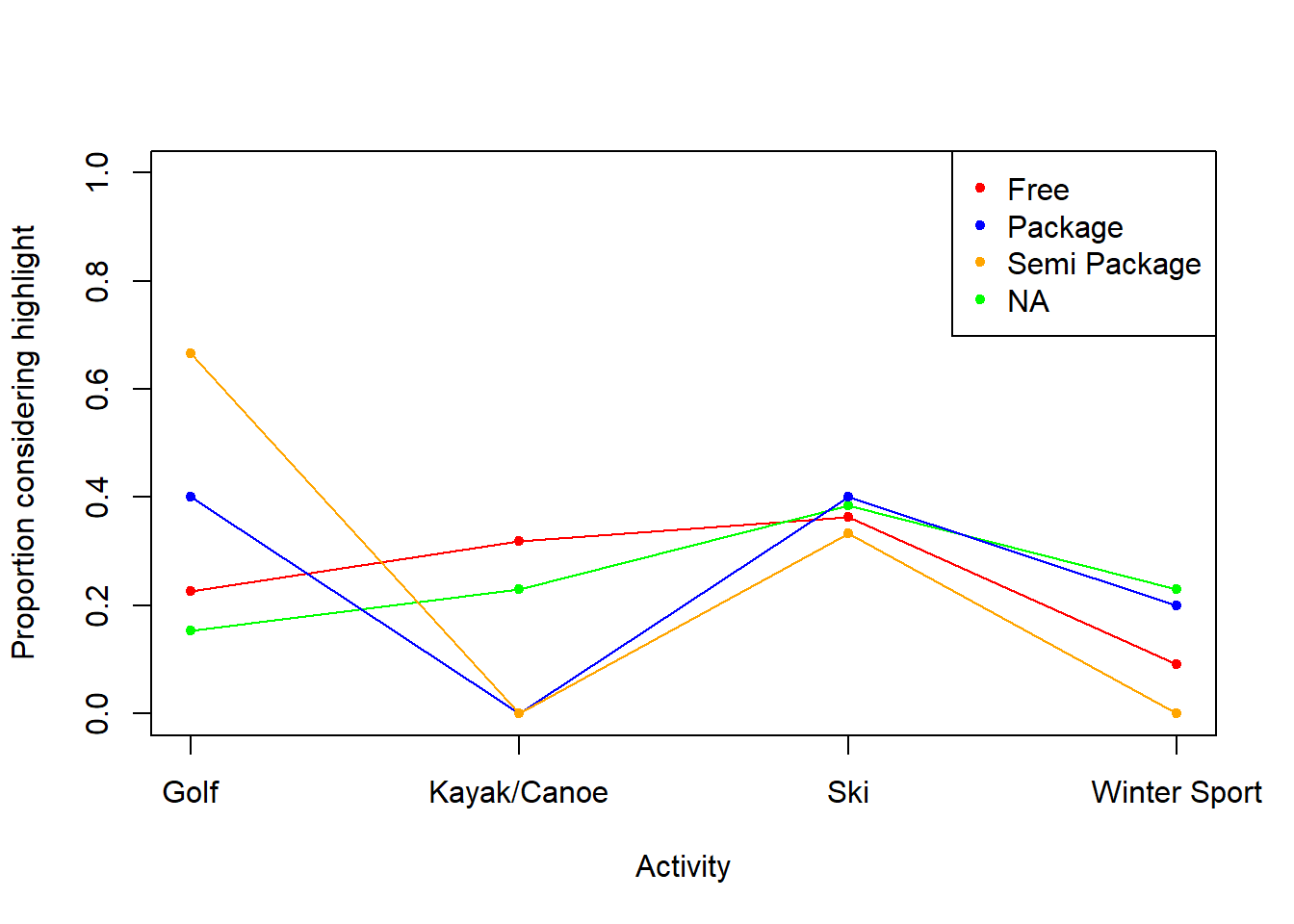

None of the surveyed Japanese tourists on a package or semi-package tour considered kayak/canoe a trip highlight, compared to more than 20% of those with a free or unspecified travel style. It may be that the tours do not typically include kayaking, but it may be worthwhile for them to add this activity as it seems well received by those who do it.

Repeat for other summary categories.

Repeat this exercise for the Australian and German tourist data.

Important Information

6d. For Loops

It is a little more challenging to group across the binary highlight variables (beginning with h) while maintaining their logistic nature. We will use a for() loop, and indicate an overall highlight (after_japan$hAdventure=1) rating for a category if more than half of the variables within it were considered highlights by each respondent.

Code

#base variable where all values are 0
after_japan$hAdventure<-c(rep(0,nrow(after_japan)))

#for each respondent
for(i in 1:nrow(after_japan)){
  temp<-c(after_japan$hRaft[i],after_japan$hJetBoat[i],after_japan$hBungy[i],after_japan$hParachute[i])
  #check if sum of binary values is greater than or equal to half the number of variables
  if(sum(temp,na.rm=T)>=(length(temp)/2)){
    #if so, change value to 1 (category was highlight)
    after_japan$hAdventure[i]<-1
  }
}

Adapt this loop for the other categories.

Code

#base variable where all values are 0
after_japan$hAdventure<-c(rep(0,nrow(after_japan)))

#for each respondent
for(i in 1:nrow(after_japan)){
  temp<-c(after_japan$hRaft[i],after_japan$hJetBoat[i],after_japan$hBungy[i],after_japan$hParachute[i])
  #check if sum of binary values is greater than or equal to half the number of variables
  if(sum(temp,na.rm=T)>=(length(temp)/2)){
    #if so, change value to 1 (category was highlight)
    after_japan$hAdventure[i]<-1
  }
}

Code

#base variable where all values are 0
after_japan$hWater<-c(rep(0,nrow(after_japan)))

#for each respondent
for(i in 1:nrow(after_japan)){
  temp<-c(after_japan$hDolphinSwim[i]+after_japan$hSwim[i]+
    after_japan$hBoatTour[i]+after_japan$hMarine[i]+after_japan$hSunbathe[i])
  #check if sum of binary values is greater than or equal to half the number of variables
  if(sum(temp,na.rm=T)>=(length(temp)/2)){
    #if so, change value to 1 (category was highlight)
    after_japan$hWater[i]<-1
  }
}

Code

#base variable where all values are 0
after_japan$hNature<-c(rep(0,nrow(after_japan)))

#for each respondent
for(i in 1:nrow(after_japan)){
  temp<-c(after_japan$hShortWalk[i]+after_japan$`hHike/Tramp`[i]+
after_japan$`hHunt/Fish`[i]+after_japan$hScenicFlight[i]+after_japan$hBotanicGarden[i]
+after_japan$hBirdWatch[i]+after_japan$hGlacier[i]+after_japan$hFarmstay[i])
  #check if sum of binary values is greater than or equal to half the number of variables
  if(sum(temp,na.rm=T)>=(length(temp)/2)){
    #if so, change value to 1 (category was highlight)
    after_japan$hNature[i]<-1
  }
}

Code

#base variable where all values are 0
after_japan$hCultural<-c(rep(0,nrow(after_japan)))

#for each respondent
for(i in 1:nrow(after_japan)){
  temp<-c(after_japan$`hMuseum/Gallery`[i]+after_japan$hCulturalPerform[i]+
  after_japan$hMarae[i]+after_japan$hHistoric[i]+after_japan$hLocals[i]+
    after_japan$hSightSeeTour[i]+after_japan$hCuisine[i])
  #check if sum of binary values is greater than or equal to half the number of variables
  if(sum(temp,na.rm=T)>=(length(temp)/2)){
    #if so, change value to 1 (category was highlight)
    after_japan$hCultural[i]<-1
  }
}

Code

#base variable where all values are 0
after_japan$hSport<-c(rep(0,nrow(after_japan)))

#for each respondent
for(i in 1:nrow(after_japan)){
  temp<-c(after_japan$`hKayak/Canoe`[i]+after_japan$hWinterSport[i]+
            after_japan$hSki[i]+after_japan$hGolf[i])
  #check if sum of binary values is greater than or equal to half the number of variables
  if(sum(temp,na.rm=T)>=(length(temp)/2)){
    #if so, change value to 1 (category was highlight)
    after_japan$hSport[i]<-1
  }
}

Code

#base variable where all values are 0
after_japan$hCity<-c(rep(0,nrow(after_japan)))

#for each respondent
for(i in 1:nrow(after_japan)){
  temp<-c(after_japan$hShop[i]+after_japan$hEveningEntertainment[i]+
after_japan$hSpecialEvent[i]+after_japan$hShows[i]+after_japan$hCasino[i])
  #check if sum of binary values is greater than or equal to half the number of variables
  if(sum(temp,na.rm=T)>=(length(temp)/2)){
    #if so, change value to 1 (category was highlight)
    after_japan$hCity[i]<-1
  }
}

This can be repeated for the Australian and German tourist data.

Important Information

6e. Contingency Table, Odds Ratios

Create a table that summarises the consideration of the summary categories as overall highlights for Japanese tourists. Make sure to include row and column totals, and informative dimension names.

Calculate the odds of each category being considered a highlight, and pick some categories to directly compare using odds ratios.

Which types of activities seem to be most popular for Japanese tourists?

Code

#wide to long, specify columns that contain binary highlight ratings for the relevant summary categories
japanLongF<-gather(data=after_japan,key="Highlights",value="Rating",c(116,117,118,119,120,121))

#table of summary categories, 0=not highlight, 1=highlight
k<-addmargins(table(japanLongF$Rating,japanLongF$Highlights))

#nice table
kable(k)

Code

#Odds of city category being considered a highlight
52/384

Code

#wide to long, specify columns that contain binary highlight ratings for the relevant summary categories
japanLongF<-gather(data=after_japan,key="Highlights",value="Rating",c(116,117,118,119,120,121))

#table of summary categories, 0=not highlight, 1=highlight
k<-addmargins(table(japanLongF$Rating,japanLongF$Highlights))

#nice table
kable(k)

	hAdventure	hCity	hCultural	hNature	hSport	hWater	Sum
0	416	384	302	273	405	352	2132
1	20	52	134	163	31	84	484
Sum	436	436	436	436	436	436	2616

Code

#Odds of city category being considered a highlight
52/384

[1] 0.1354167

Code

#adventure
20/416

[1] 0.04807692

Code

#cultural
134/302

[1] 0.4437086

Code

#nature
163/273

[1] 0.5970696

Code

#sport
31/405

[1] 0.07654321

Code

#water
84/352

[1] 0.2386364

Code

#odds ratio, nature over cultural
OR<-(163/273)/(134/302)
OR

[1] 1.345634

The two categories most likely to be considered trip highlights are cultural and nature activities. For Japanese tourists, the odds of considering nature based activities to be trip highlights are 1.345 times the odds of considering cultural activities to be trip highlights.

These findings suggest that New Zealand tourism advertising for the Japanese market should emphasise the natural environment (mountains, lakes, bush scenery) and activities that involve this.

This can be repeated for the Australian and German tourist data.

Important Information

Consider some issues with surveys as a method of data collection. How might these impact the conclusions we can make from this analysis?

Tourists (potential and previous) who responded to the survey could differ in many ways from those that did not e.g. demographic characteristics, chosen tour structure, overall satisfaction/dissatisfaction with trip. As a result, the findings of this analysis may not be representative of the entire population of tourists from Japan, Germany or Australia.

Tourists from different countries may also systematically differ in how they rate items or respond to surveys, which could bias the results when carrying out comparisons. For example, Japanese tourists may consider it polite to give all activities a moderate rating even if they did not particularly enjoy them. Tourists from Australia or Germany may give more dramatic ratings, exaggerating satisfaction or dissatisfaction.

Self-report of survey answers can also affect the quality of data. Tourists who visited New Zealand some time ago may have forgotten or misremembered details, resulting in an inaccurate representation of their experiences.