17 Takahē Hatching

The Takahē is a flightless, endangered bird that is endemic to New Zealand (meaning that it is only found here). The Takahē used to be widespread over the country, however in the present day the only colony in a natural habitat is in Fiordland, in the lower South Island. The New Zealand Department of Conservation run a management program to monitor and protect the remaining population: some birds were translocated to islands around New Zealand, which are thought of as refuges or safe-havens for the Takahē. The Takahē are monitored on these islands, and as part of the program to help increase their population size, breeding activity is closely monitored in effort to isolate some of the issues that result in the limited breeding success.

The main hypothesis presented for this data set and the aim of this lesson is to investigate whether human disturbance of the nests (to monitor the breeding) affects breeding success (compared to the breeding success of nests without human disturbance).

Data

Data Summary

29 observations

10 variables

Variable	Type	Information
Females	Categorical	5 levels: Bunchy, Puffin, Terri, Toni & Tilly, Toru, Vicky, Bar. Name of female(s) in nest.
Year	Continuous
Treatment	Categorical	2 levels: D (disturbed), ND (non-disturbed).
No. eggs	Discrete
Eggs missing	Discrete
No. fertile	Discrete	Fertile eggs.
No. infertile	Discrete	Infertile eggs.
No. dead embryos	Discrete
No. hatch	Discrete	Chicks that hatch.
No. fledge	Discrete	Chicks that fledge.

There is 1 data file associated with this presentation. It contains the data you will need to complete the lesson tasks.

Download TakaheDataAndVariables.xls

Video

Important Information

This lesson uses analysis techniques for both count (proportion) and continuous data. Most of these have been explored in previous lessons so the code is initially hidden. It is recommended you leave the tasks below until after you have worked through the other lessons. These tasks can then function as revision exercises to help you recall the relevant techniques.

Objectives

Learning Objectives

This lesson provides the opportunity to recall and practice analysis techniques that have been previously demonstrated.

Reinforcing skills and concepts seen in earlier lessons:

Data wrangling - read data, recode and rename variables, new variables.
Data consolidation - response by levels of predictor.
Hypothesis tests - small sample.
Bootstrap confidence interval - means, difference in means.
Plotting - histograms.

Tasks

0. Read and Format data

0a. Read in the data

First make sure you have installed the package readxl and set the working directory, using instructions in Getting started with R Section 2.6.

Load the data into R.

Important Information

Name your data nesting for easier reference later.

The code has been hidden initially, so you can try to load the data yourself first before checking the solutions.

Code

library(readxl) #loads readxl package

nesting<-read_xls("TakaheDataAndVariables.xls",range="A1:K30") #loads the data file and names it nesting

head(nesting) #view beginning of data frame

Code

library(readxl) #loads readxl package

Warning: package 'readxl' was built under R version 4.2.2

Code

nesting<-read_xls("TakaheDataAndVariables.xls",range="A1:K30") #loads the data file and names it nesting

head(nesting) #view beginning of data frame

# A tibble: 6 × 11
  Females   Year Treat…¹ No. e…² Eggs …³ No.  …⁴ No.  …⁵ No. d…⁶ No. h…⁷ No. f…⁸
  <chr>    <dbl> <chr>     <dbl>   <dbl>   <dbl>   <dbl>   <dbl>   <dbl>   <dbl>
1 Bunchy    2000 D             1      NA       0       1       0       0      NA
2 Puffin    2000 D             2      NA       2       0       2       0      NA
3 Terri     2000 D             1      NA       1       0       0       1       1
4 Toni&Ti…  2000 ND            3      NA       2       1       2       0      NA
5 Toru      2000 ND            1      NA       1       0       0       1       1
6 Vicky     2000 ND            1      NA       1       0       1       0      NA
# … with 1 more variable: Comments <chr>, and abbreviated variable names
#   ¹Treatment, ²`No. eggs*`, ³`Eggs missing`, ⁴`No.  fertile*`,
#   ⁵`No.  Infertile*`, ⁶`No. dead embryos`, ⁷`No. hatch`, ⁸`No. fledge`
# ℹ Use `colnames()` to see all variable names

This opens a data frame from a study investigating the success of different stages of the breeding cycle of Takahē in non-disturbed and disturbed habitats.

The variables recorded are Females (the names of the female Takahē in each pair), Year, Treatment (D = disturbed, ND = not disturbed), No.eggs (number of eggs observed), Eggs missing (the number of eggs that were missed in the count), No.fertile, No.Infertile, No.dead embryos, No.hatch (number of eggs that hatched), No.fledge (number of eggs that fledged) and Comments (other information).

0b. Format the data

R has automatically loaded all variables in the data frame as character vectors, however they are a combination of factors and numeric variables.

Recode the variables as their correct classification and rename them to remove spaces.

Code

#recoding as factors
nesting$Females<-as.factor(nesting$Females)
nesting$Treatment<-as.factor(nesting$Treatment)

#renaming columns for easier reference
colnames(nesting)<-c("Females","Year","Treatment","No.eggs","Eggs.missing","No.fertile","No.infertile","No.deadembryos","No.hatch","No.fledge","Comments")

Code

#recoding as factors
nesting$Females<-as.factor(nesting$Females)
nesting$Treatment<-as.factor(nesting$Treatment)

#renaming columns for easier reference
colnames(nesting)<-c("Females","Year","Treatment","No.eggs","Eggs.missing","No.fertile","No.infertile","No.deadembryos","No.hatch","No.fledge","Comments")

In this study 8 pairs of Takahē (male-female) were monitored and different stages of their breeding success were monitored. As the sample size was so small it was unrealistic to allocate half the pairs to the non-disturbed group and the other half to the disturbed group. Because of this a matched-pairs design was employed. This means that the breeding pairs alternated between treatment (disturbed nests) and control (non-disturbed nests) over four seasons (i.e. each year the treatments swap over for each pair).

1. Calculate Proportions

Calculate the average hatching success and fertility percentages for the non-disturbed and disturbed nests.

Calculate the differences between these proportions for hatching success and fertility and report any tentative conclusions that you make.

First calculate new columns with the hatching success proportion (No.hatch/No.eggs) and fertility proportion (No.fertile/No.eggs) for each breeding pair.

Code

nesting$P.hatch<-nesting$No.hatch/nesting$No.eggs #hatching success
nesting$P.fertile<-nesting$No.fertile/nesting$No.eggs #fertility

Then calculate the average P.hatch for the non-disturbed and disturbed pairs using tapply()

Code

tapply(nesting$P.hatch,INDEX=nesting$Treatment,FUN=mean,na.rm=T) #remove NAs to avoid errors

Modify this code to find the average P.fertile for non-disturbed and disturbed pairs.

Code

nesting$P.hatch<-nesting$No.hatch/nesting$No.eggs #hatching success
nesting$P.fertile<-nesting$No.fertile/nesting$No.eggs #fertility

Code

tapply(nesting$P.hatch,INDEX=nesting$Treatment,FUN=mean,na.rm=T) #remove NAs to avoid errors

        D        ND 
0.4508242 0.7038462

Code

tapply(nesting$P.fertile,INDEX=nesting$Treatment,FUN=mean,na.rm=T) #remove NAs to avoid errors

        D        ND 
0.7499084 0.8705128

The proportion of hatched eggs is 0.253022 (or approximately 25%) higher for non-disturbed nests. The proportion of fertile eggs is 0.1206044 (or approximately 12%) higher for non-disturbed nests.

These results seem to suggest that the eggs of non-disturbed nests fare better than those in nests which are disturbed by researchers. However, in order to make conclusions we must consider the uncertainty/variability around these point estimates.

2. Non-Parametric T-Test

Carry out a non-parametric Wilcoxon matched pairs test on the proportions found above for fertility, hatching success, and fecundity (No.eggs).

Important Information

Non-parametric procedures are required for this data set (as opposed to a paired t-test) due to the small sample sizes and type of data recorded.

Report the findings and state any conclusions.

The function wilcox.test() is used in much the same way as t.test(), have a look at the help file for some tips.

Code

wilcox.test(nesting$P.fertile[nesting$Treatment=="D"],nesting$P.fertile[nesting$Treatment=="ND"],paired=TRUE) #since the data are matched, we set paired=TRUE

Carry out this Wilcoxon test for the P.hatch and the *No.eggs pairs and report your findings

Code

wilcox.test(nesting$P.fertile[nesting$Treatment=="D"],nesting$P.fertile[nesting$Treatment=="ND"],paired=TRUE) #since the data are matched, we set paired=TRUE

Warning in wilcox.test.default(nesting$P.fertile[nesting$Treatment == "D"], :
cannot compute exact p-value with ties

Warning in wilcox.test.default(nesting$P.fertile[nesting$Treatment == "D"], :
cannot compute exact p-value with zeroes


    Wilcoxon signed rank test with continuity correction

data:  nesting$P.fertile[nesting$Treatment == "D"] and nesting$P.fertile[nesting$Treatment == "ND"]
V = 8, p-value = 0.3517
alternative hypothesis: true location shift is not equal to 0

Code

wilcox.test(nesting$P.hatch[nesting$Treatment=="D"],nesting$P.hatch[nesting$Treatment=="ND"],paired=TRUE) #since the data are matched, we set paired=TRUE

Warning in wilcox.test.default(nesting$P.hatch[nesting$Treatment == "D"], :
cannot compute exact p-value with ties

Warning in wilcox.test.default(nesting$P.hatch[nesting$Treatment == "D"], :
cannot compute exact p-value with zeroes


    Wilcoxon signed rank test with continuity correction

data:  nesting$P.hatch[nesting$Treatment == "D"] and nesting$P.hatch[nesting$Treatment == "ND"]
V = 8, p-value = 0.1813
alternative hypothesis: true location shift is not equal to 0

Code

wilcox.test(nesting$No.eggs[nesting$Treatment=="D"],nesting$No.eggs[nesting$Treatment=="ND"],paired=TRUE) #since the data are matched, we set paired=TRUE

Warning in wilcox.test.default(nesting$No.eggs[nesting$Treatment == "D"], :
cannot compute exact p-value with ties

Warning in wilcox.test.default(nesting$No.eggs[nesting$Treatment == "D"], :
cannot compute exact p-value with zeroes


    Wilcoxon signed rank test with continuity correction

data:  nesting$No.eggs[nesting$Treatment == "D"] and nesting$No.eggs[nesting$Treatment == "ND"]
V = 35, p-value = 0.1475
alternative hypothesis: true location shift is not equal to 0

The wilcoxon test comparing the proportion of fertile eggs in the disturbed and non-disturbed nests returns a test statistic of 8, with an associated p-value of 0.3517. This is greater than 0.05 and therefore indicates no significant evidence of a difference in the proportion of fertile eggs. There is a reasonable chance of observing the difference in our sample under the null hypothesis of no true population difference. Although the point estimates (discussed in Task 1) are not very similar for the disturbed and non-disturbed nests, due to the small sample size there is quite a large margin of error around them and the population values may be a lot closer.

Analogous conclusions can be made for the proportion of hatched eggs and the number of eggs, these wilcoxon tests also returned non-significant p-values. The small sample size limits the power of the test, that is, our ability to determine a true difference if one does exist.

3. Bootstrap Confidence Interval (mean)

Perform a bootstrap for the mean number of hatched eggs (No.hatch) for the non-disturbed and disturbed nests. Calculate the accompanying 95% confidence intervals and plot these on histograms of the bootstrapped results.

The bootstrapping technique is especially useful for data sets that have a small number of actual samples, such as the Takahē data set that we are working with now.

Perform bootstrap

Code

library(boot)

#set seed so you get the same results when running again
set.seed(41)   

#function that calculates the mean from the bootstrapped samples
meanFun<-function(data,indices){  
  dataInd<-data[indices,]
  meandata<-mean(dataInd$No.hatch,na.rm=T)
  return(meandata)
}

#bootstrap mean number of eggs hatched in non-disturbed nests.
#Create object called meanBoot with the output of the bootstrapping procedure
meanBoot<-boot(nesting[nesting$Treatment=="D",],statistic=meanFun, R=10000)

Check summary results

Code

#view bootstrap output
meanBoot

Construct confidence interval of your choice

Code

#percentile confidence interval
percCi<-boot.ci(meanBoot,type="perc") 

#check lower and upper limits from percentile interval object
percCi$percent[4:5]

Plot histogram of results, with density curve and confidence interval limits superimposed

Code

#plot density histogram of bootstrap results
hist(meanBoot$t,breaks=20,freq=F, main="Mean number of Takahe hatched in Disturbed Nests") 

#add a smoothed line to show the distribution
lines(density(meanBoot$t),col="darkslategray3",lwd=2) 

#ci limits
abline(v=percCi$percent[4:5],col="darkslategray4",lty=2)

Repeat this bootstrap procedure for the number of hatched eggs in non-disturbed nests and report your findings.

First carry out the bootstrap procedure for disturbed nests, and plot the results.

Code

library(boot)

Warning: package 'boot' was built under R version 4.2.2

Code

#set seed so you get the same results when running again
set.seed(41)   

#function that calculates the mean from the bootstrapped samples
meanFun<-function(data,indices){  
  dataInd<-data[indices,]
  meandata<-mean(dataInd$No.hatch,na.rm=T)
  return(meandata)
}

#bootstrap mean number of eggs hatched in disturbed nests.
#Create object called meanBoot with the output of the bootstrapping procedure
meanBoot<-boot(nesting[nesting$Treatment=="D",],statistic=meanFun, R=10000)

Code

#view bootstrap output
meanBoot


ORDINARY NONPARAMETRIC BOOTSTRAP


Call:
boot(data = nesting[nesting$Treatment == "D", ], statistic = meanFun, 
    R = 10000)


Bootstrap Statistics :
    original       bias    std. error
t1* 1.307692 -0.002202112   0.2533887

Code

#percentile confidence interval
percCi<-boot.ci(meanBoot,type="perc") 

#check lower and upper limits from percentile interval object
percCi$percent[4:5]

[1] 0.800000 1.785714

Code

#plot density histogram of bootstrap results
hist(meanBoot$t,breaks=20,freq=F, main="Mean number of Takahe hatched in Disturbed Nests") 

#add a smoothed line to show the distribution
lines(density(meanBoot$t),col="darkslategray3",lwd=2) 

#ci limits
abline(v=percCi$percent[4:5],col="darkslategray4",lty=2)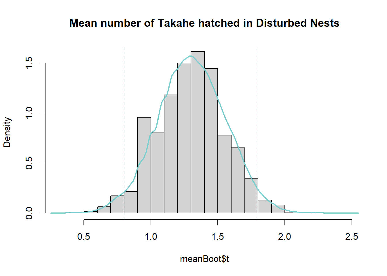

The bootstrapped means for the number of hatched eggs in the disturbed nests follow a normal distribution symmetric around a mean of 1.307692. This mean of means matches the actual mean number of hatched eggs in the disturbed nests, and the distribution of bootstrapped mean estimates around it give an indication of the amount of variability in our estimate due to sampling.

We can be 95% confident the true mean number of hatches for non-disturbed nests lies between 0.800000 and 1.785714, that is, less than 1 per nest to slightly under 2 per nest.

Some slight modifications to the code above allow construction of a bootstrap for non-disturbed nests.

Code

library(boot)

#set seed so you get the same results when running again
set.seed(41)   

#function that calculates the mean from the bootstrapped samples
meanFun<-function(data,indices){  
  dataInd<-data[indices,]
  meandata<-mean(dataInd$No.hatch,na.rm=T)
  return(meandata)
}

#bootstrap mean number of eggs hatched in non-disturbed nests.
#Create object called meanBoot with the output of the bootstrapping procedure
meanBoot<-boot(nesting[nesting$Treatment=="ND",],statistic=meanFun, R=10000)

Code

#view bootstrap output
meanBoot


ORDINARY NONPARAMETRIC BOOTSTRAP


Call:
boot(data = nesting[nesting$Treatment == "ND", ], statistic = meanFun, 
    R = 10000)


Bootstrap Statistics :
    original       bias    std. error
t1* 1.307692 -0.005205721   0.2309913

Code

#percentile confidence interval
percCi<-boot.ci(meanBoot,type="perc") 

#check lower and upper limits from percentile interval object
percCi$percent[4:5]

[1] 0.8571429 1.7692308

Code

#plot density histogram of bootstrap results
hist(meanBoot$t,breaks=20,freq=F, main="Mean number of Takahe hatched in Non-Disturbed Nests") 

#add a smoothed line to show the distribution
lines(density(meanBoot$t),col="darkslategray3",lwd=2) 

#ci limits
abline(v=percCi$percent[4:5],col="darkslategray4",lty=2)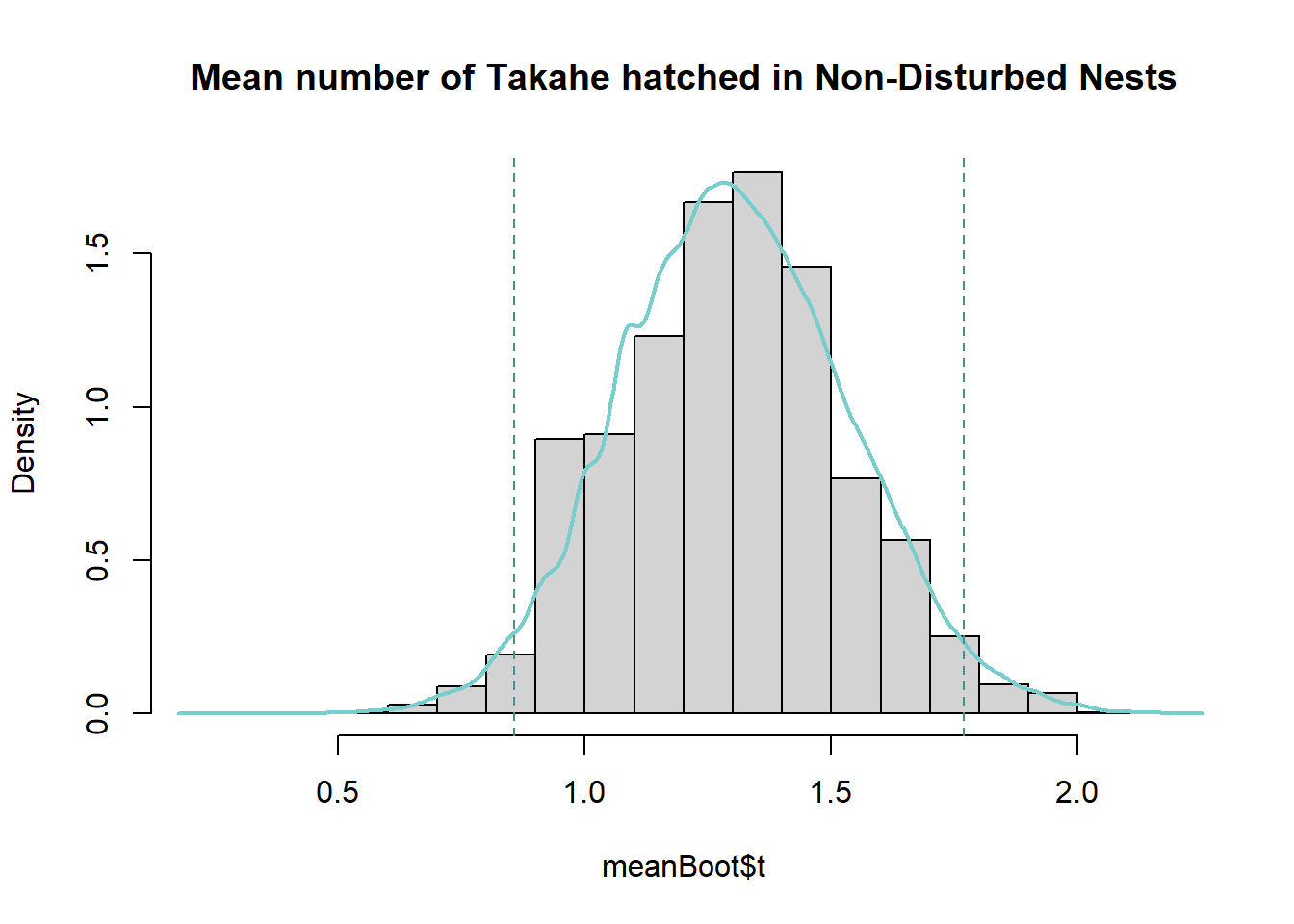

The bootstrapped means for the number of hatched eggs in the non-disturbed nests follow a normal distribution symmetric around a mean of 1.307692. This mean of means matches the actual mean number of hatched eggs in the non-disturbed nests, and the distribution of bootstrapped mean estimates around it give an indication of the amount of variability in our estimate due to sampling. We can be 95% confident the true mean number of hatches for non-disturbed nests lies between 0.8571429 and 1.7692308, that is, less than 1 per nest to slightly under 2 per nest.

Note that while observed mean number of hatches is the same for the disturbed and non-disturbed nests, there is reduced variability around this estimate for the non-disturbed nests.

4. Bootstrap Confidence Interval (difference in means)

Calculate the mean and confidence interval for the difference between the number of hatched eggs (No.hatch) in the disturbed and non-disturbed groups, using the bootstrap procedure.

Report your findings along with an appropriate plot, and discuss your conclusions with reference to the previous questions.

What distribution does the bootstrap sampling appear to follow? Why do you think this is the case?

Code

library(boot)

#set seed so you get the same results when running again
set.seed(42) 

#function that calculates the difference in means from the bootstrapped samples
meandiffFun<-function(data,indices){  
  data1<-data[data$Treatment=="D",] #subset data by treatment levels, then sample from these
  dataInd1<-data1[indices,]
  data2<-data[data$Treatment=="ND",] #subset data by treatment levels, then sample from these
  dataInd2<-data2[indices,]
  meandiff<-mean(dataInd1$No.hatch,na.rm=T)-mean(dataInd2$No.hatch,na.rm=T) #calculate difference in means for the samples. Use na.rm=T to remove NAs
  return(meandiff)
}

#bootstrap difference in mean number of hatched eggs for disturbed and non-disturbed Takahe nests.
#create object called meandiffBoot with the output of the bootstrapping procedure
meandiffBoot<-boot(nesting[nesting$Treatment=="D"|nesting$Treatment=="ND",],statistic=meandiffFun, R=10000)

Code

#view bootstrap output
meandiffBoot

Code

#percentile confidence interval
percCi<-boot.ci(meandiffBoot,type="perc") 

#check lower and upper limits from percentile interval object
percCi$percent[4:5]

Code

#plot density histogram of bootstrap results
hist(meandiffBoot$t,breaks=20,freq=F, main="Difference in Mean number of Takahe hatched \n in Disturbed - Non-Disturbed Nests") 

#add a smoothed line to show the distribution
lines(density(meandiffBoot$t),col="darkslategray3",lwd=2) 

#ci limits
abline(v=percCi$percent[4:5],col="darkslategray4",lty=2)

Code

library(boot)

#set seed so you get the same results when running again
set.seed(42) 

#function that calculates the difference in means from the bootstrapped samples
meandiffFun<-function(data,indices){  
  data1<-data[data$Treatment=="D",] #subset data by treatment levels, then sample from these
  dataInd1<-data1[indices,]
  data2<-data[data$Treatment=="ND",] #subset data by treatment levels, then sample from these
  dataInd2<-data2[indices,]
  meandiff<-mean(dataInd1$No.hatch,na.rm=T)-mean(dataInd2$No.hatch,na.rm=T) #calculate difference in means for the samples. Use na.rm=T to remove NAs
  return(meandiff)
}

#bootstrap difference in mean number of hatched eggs for disturbed and non-disturbed Takahe nests.
#create object called meandiffBoot with the output of the bootstrapping procedure
meandiffBoot<-boot(nesting[nesting$Treatment=="D"|nesting$Treatment=="ND",],statistic=meandiffFun, R=10000)

Code

#view bootstrap output
meandiffBoot


ORDINARY NONPARAMETRIC BOOTSTRAP


Call:
boot(data = nesting[nesting$Treatment == "D" | nesting$Treatment == 
    "ND", ], statistic = meandiffFun, R = 10000)


Bootstrap Statistics :
    original        bias    std. error
t1*        0 -0.0002252258   0.2968207

Code

#percentile confidence interval
percCi<-boot.ci(meandiffBoot,type="perc") 

#check lower and upper limits from percentile interval object
percCi$percent[4:5]

[1] -0.5960784  0.5768939

Code

#plot density histogram of bootstrap results
hist(meandiffBoot$t,breaks=20,freq=F, main="Difference in Mean number of Takahe hatched \n in Disturbed - Non-Disturbed Nests") 

#add a smoothed line to show the distribution
lines(density(meandiffBoot$t),col="darkslategray3",lwd=2) 

#ci limits
abline(v=percCi$percent[4:5],col="darkslategray4",lty=2)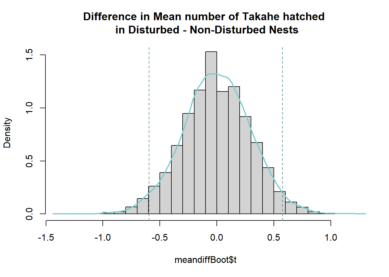

The bootstrapped difference in means for the number of hatched eggs between disturbed and non-disturbed nests follows a normal distribution symmetric around a mean of 0. This mean difference in means matches the actual difference in mean number of hatched eggs in the disturbed and non-disturbed nests, and the distribution of bootstrapped difference in mean estimates around it give an indication of the amount of variability due to sampling. We can be 95% confident the true difference in mean number of hatches for disturbed and non-disturbed nests lies between -0.5960784 and 0.5768939. That is, disturbed nests on average could hatch anywhere from half an egg more to half an egg less than non-disturbed nests.

As the confidence interval for the difference in means includes 0 we cannot make a conclusion regarding the direction of the true difference in mean number of hatched eggs for disturbed vs non-disturbed nests. It could be greater for disturbed, less for disturbed, or equal between disturbed and non-disturbed. These findings are what we would expect based on results from the wilcoxon test in Task 2 - there was no significant evidence of a difference in either the proportion of eggs that hatched or the number of eggs that were laid between the disturbed and non-disturbed nests.

The bootstrapped samples follow a normal distribution, as would be expected according to the Central Limit Theorem (CLT). The CLT states that the distribution of means of random variables will converge to a normal distribution as the sample size approaches infinity (for example, in a bootstrap with 10,000 samples).