16 Aviation Accidents and Incidents

This lesson uses studies of aviation events to demonstrate techniques for data where both the predictor and response variables take categorical values. Performance shaping factors affecting aircraft accidents (serious events) and incidents (minor events) should be investigated in order to reduce the possibility of future accidents. This study, presented by David O’Hare, investigates human behaviours which may be involved in such accidents and incidents.

Data

Data Summary

1144 observations

14 variables

Variable	Type	Information
age	Continuous	Years.
hrstot	Continuous	Total number of flight hours.
event_type	Categorical	3 levels: 0 (no event), 1 (incident), 2 (accident).
failure_mode	Categorical	7 levels: 1 (mechanical), 2 (information), 3 (diagnosis), 4 (goal), 5 (strategy), 6 (procedure).
p_distract	Categorical	Person distraction, 2 levels: 1 (yes), 2 (no).
othr_distract	Categorical	Other distraction, 2 levels: 1 (yes), 2 (no).
workload	Categorical	Workload excessive, 2 levels: 1 (yes), 2 (no).
interfnc	Categorical	Interference of one task with another, 2 levels: 1 (yes), 2 (no).
nontrn	Categorical	Lack of training, 2 levels: 1 (yes), 2 (no).
wrngtrn	Categorical	Faulty training, 2 levels: 1 (yes), 2 (no).
incapac	Categorical	Physically incapacitated, 2 levels: 1 (yes), 2 (no).
mentals	Categorical	Mental state affected, 2 levels: 1 (yes), 2 (no).
int_physical	Categorical	Cockpit environment, 2 levels: 1 (yes), 2 (no).
ext_physical	Categorical	External environment, 2 levels: 1 (yes), 2 (no).

There are 2 files associated with this presentation. The first contains the data you will need to complete the lesson tasks, and the second contains descriptions of the variables included in the data file.

Download AircraftData.xls

Download AircraftVariables.xls

Video

Objectives

Learning Objectives

New skills and concepts:

Self-report data.
\(\chi^2\) tests.

Reinforcing skills and concepts seen in earlier lessons:

Read and format data.
Cross-tabulation (count and proportion).
Bar plots.
Multiple logistic regression.

Tasks

0. Read and Format data

0a. Read in the data

First make sure you have installed the package readxl (see Section 2.6) and set the working directory (see Section 2.1).

Load the data into R.

Important Information

Name your data aircraft for easier reference later.

Previous Lesson

To load the data in R we run code analogous to Task 0 in Cockles Section 3.0.1

The code has been hidden initially, so you can try to load the data yourself first before checking the solutions.

Code

#loads readxl package
library(readxl)

#loads the data file and names it aircraft
aircraft<-read_xls("AircraftData.xls") 

#view beginning of data frame
head(aircraft)

Code

#loads readxl package
library(readxl)

Warning: package 'readxl' was built under R version 4.2.2

Code

#loads the data file and names it aircraft
aircraft<-read_xls("AircraftData.xls") 

#view beginning of data frame
head(aircraft)

# A tibble: 6 × 14
    age hrstot event_type failu…¹ p_dis…² othr_…³ workl…⁴ inter…⁵ nontrn wrngtrn
  <dbl>  <dbl>      <dbl>   <dbl>   <dbl>   <dbl>   <dbl>   <dbl>  <dbl>   <dbl>
1    60   1600          1       1       2       2       1       2      2       2
2    26     80          0      NA       0       0       0       0      0       0
3    34     82          0      NA       0       0       0       0      0       0
4    59    230          0      NA       0       0       0       0      0       0
5    41  11000          0      NA       0       0       0       0      0       0
6    45    286          0      NA       0       0       0       0      0       0
# … with 4 more variables: incapac <dbl>, mentals <dbl>, int_physical <dbl>,
#   ext_physical <dbl>, and abbreviated variable names ¹failure_mode,
#   ²p_distract, ³othr_distract, ⁴workload, ⁵interfnc
# ℹ Use `colnames()` to see all variable names

This opens the “AircraftData.xls” dataset. This dataset contains information on performance shaping factors and the resulting events in 1144 reports from aircraft pilots.

0b. Format the data

Many of the variables in this data set are binary (categorical with 2 levels). They are currently coded as 1 (yes) and 2 (no), but it is easier to work with binary data coded as 1 (yes) and 0 (no).

Recode the relevant categorical variables.

Code

#overwrite entries equal to 2 (no) with 0 (binary no)
aircraft$p_distract[aircraft$p_distract==2]<-0

Repeat for other binary variables.

Code

#overwrite entries equal to 2 (no) with 0 (binary no)
aircraft$p_distract[aircraft$p_distract==2]<-0

Code

#overwrite entries equal to 2 (no) with 0 (binary no)
aircraft$othr_distract[aircraft$othr_distract==2]<-0

Code

#overwrite entries equal to 2 (no) with 0 (binary no)
aircraft$workload[aircraft$workload==2]<-0

Code

#overwrite entries equal to 2 (no) with 0 (binary no)
aircraft$interfnc[aircraft$interfnc==2]<-0

Code

#overwrite entries equal to 2 (no) with 0 (binary no)
aircraft$nontrn[aircraft$nontrn==2]<-0

Code

#overwrite entries equal to 2 (no) with 0 (binary no)
aircraft$wrngtrn[aircraft$wrngtrn==2]<-0

Code

#overwrite entries equal to 2 (no) with 0 (binary no)
aircraft$incapac[aircraft$incapac==2]<-0

Code

#overwrite entries equal to 2 (no) with 0 (binary no)
aircraft$mentals[aircraft$mentals==2]<-0

Code

#overwrite entries equal to 2 (no) with 0 (binary no)
aircraft$int_physical[aircraft$int_physical==2]<-0

Code

#overwrite entries equal to 2 (no) with 0 (binary no)
aircraft$ext_physical[aircraft$ext_physical==2]<-0

Code

#check new data frame
head(aircraft)

# A tibble: 6 × 14
    age hrstot event_type failu…¹ p_dis…² othr_…³ workl…⁴ inter…⁵ nontrn wrngtrn
  <dbl>  <dbl>      <dbl>   <dbl>   <dbl>   <dbl>   <dbl>   <dbl>  <dbl>   <dbl>
1    60   1600          1       1       0       0       1       0      0       0
2    26     80          0      NA       0       0       0       0      0       0
3    34     82          0      NA       0       0       0       0      0       0
4    59    230          0      NA       0       0       0       0      0       0
5    41  11000          0      NA       0       0       0       0      0       0
6    45    286          0      NA       0       0       0       0      0       0
# … with 4 more variables: incapac <dbl>, mentals <dbl>, int_physical <dbl>,
#   ext_physical <dbl>, and abbreviated variable names ¹failure_mode,
#   ²p_distract, ³othr_distract, ⁴workload, ⁵interfnc
# ℹ Use `colnames()` to see all variable names

This dataset contains performance shaping factors for incidents, accidents,and situations where no event occurred. Some of the analysis carried out in the video (that we will replicate in this lesson), is interested only in the comparison between incidents and accidents (disregarding non-events).

Create a second data frame that only includes observations where an incident or accident occurred.

Code

#subset observations where event type is 1 (incident) or 2 (accident)
aircraftFailure<-aircraft[which(aircraft$event_type=="1"|aircraft$event_type=="2"),]

#check new data frame
head(aircraftFailure)

Code

#subset observations where event type is 1 (incident) or 2 (accident)
aircraftFailure<-aircraft[which(aircraft$event_type=="1"|aircraft$event_type=="2"),]

#check new data frame
head(aircraftFailure)

# A tibble: 6 × 14
    age hrstot event_type failu…¹ p_dis…² othr_…³ workl…⁴ inter…⁵ nontrn wrngtrn
  <dbl>  <dbl>      <dbl>   <dbl>   <dbl>   <dbl>   <dbl>   <dbl>  <dbl>   <dbl>
1    60   1600          1       1       0       0       1       0      0       0
2    33     90          1       1       0       0       0       0      0       0
3    41    158          1       3       0       0       0       0      1       0
4    44   3500          1       2       0       0       0       0      0       0
5    29    300          1       5       1       0       0       0      0       0
6    56    239          1       7       0       0       0       0      0       0
# … with 4 more variables: incapac <dbl>, mentals <dbl>, int_physical <dbl>,
#   ext_physical <dbl>, and abbreviated variable names ¹failure_mode,
#   ²p_distract, ³othr_distract, ⁴workload, ⁵interfnc
# ℹ Use `colnames()` to see all variable names

1. Cross-Tabulation, Bar Plot (response by predictor)

1a. Cross-Tabulation

Using the aircraftFailure data frame, construct a cross tabulation of event_type against each of the 7 categories in failure_mode.

Previous Lesson

See Epidemiology Task 1. Section 11.1.2 or Otago Stadium Task 2a. Section 12.0.3 for cross tabulation of 2 variables.

Calculate these values as proportions, that sum to 1 for each event type.

Code

#using prop.table on a table object converts the counts to proportions
#margin=1 sums over rows
prop.table(table(aircraftFailure$event_type,aircraftFailure$failure_mode),margin=1)

Code

#using prop.table on a table object converts the counts to proportions
#margin=1 sums over rows
prop.table(table(aircraftFailure$event_type,aircraftFailure$failure_mode),margin=1)

   
             1          2          3          4          5          6
  1 0.39914163 0.22317597 0.10729614 0.11587983 0.03862661 0.02145923
  2 0.31372549 0.17647059 0.07843137 0.25490196 0.07843137 0.05882353
   
             7
  1 0.09442060
  2 0.03921569

1b. Bar plot

It is often easier to compare values over many categories using visualisation. Use your table from 1a. to create a bar plot.

What does your bar plot show?

Previous Lesson

See Otago stadium Task 2b. Section 12.0.3 for bar plot creation.

Code

#store proportion values in a matrix
AIMatrix<-prop.table(table(aircraftFailure$event_type,aircraftFailure$failure_mode),margin=1)

Code

#barplot using matrix
barplot(AIMatrix,beside=TRUE,names.arg=c("Mechanical","Information","Diagnosis","Goal","Strategy","Procedure","Action"),col=c("darkorange1","red3"),ylab="Proportion",xlab="Failure Mode",main="Event type by Failure mode",ylim=c(0,0.5),cex.names=0.82)
legend("topright",c("Incident","Accident"),fill=c("darkorange1","red3"))

Code

#store proportion values in a matrix
AIMatrix<-prop.table(table(aircraftFailure$event_type,aircraftFailure$failure_mode),margin=1)

Code

#barplot
barplot(AIMatrix,beside=TRUE,names.arg=c("Mechanical","Information","Diagnosis","Goal","Strategy","Procedure","Action"),col=c("darkorange1","red3"),ylab="Proportion",xlab="Failure Mode",main="Event type by Failure mode",ylim=c(0,0.5),cex.names=0.82)
legend("topright",c("Incident","Accident"),fill=c("darkorange1","red3"))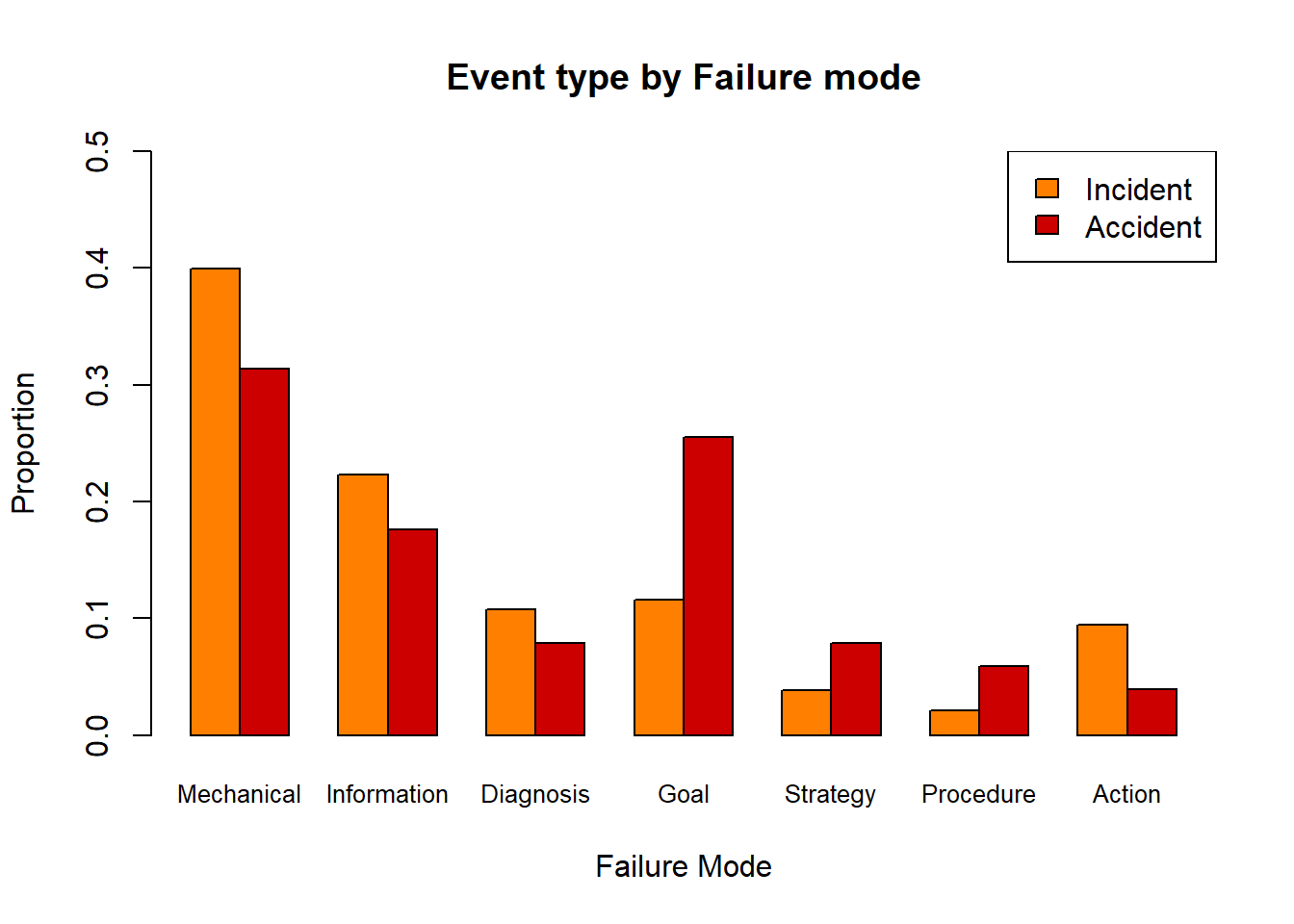

The mechanical, information, diagnosis and action failure modes are associated with a higher proportion of incidents than accidents, while the reverse is true for the goal, strategy and procedure failure modes. The goal mode has the largest difference in proportion of associated accidents and incidents.

Create cross-tabulations of the proportions of event_type associated with each of the 10 performance shaping factors (e.g. p_distract, workload, ext_physical etc.).

Following this, you can construct a matrix of proportion values of accidents and incidents associated with each performance shaping factor and replicate the bar graph shown in the video (12.58). Note - you should not plot all the values in your table so you must first make a matrix of the relevant ones, rather than provide the table directly to the barplot() function.

Previous Task

Modify the techniques used earlier in this task to create tables of proportions.

Previous Lesson

See Rejection and Self-Esteem Task 6b. Section 10.0.7 for bar plot creation from a matrix of values.

The data used for this analysis came from self-reports of pilots who responded to a survey request.

How might these factors (participant response to survey and self-report) affect the data that was collected, and therefore the conclusions that can be made?

Although pilots who responded to the survey did not differ from those that declined in terms of demographics (as addressed in the video), the characteristics of their crashes may not be the same.For example, pilots who had an accident that was attributed to their actions (e.g. diagnosis, strategy) may feel uncomfortable about publicising this information. As a result, the association between these failure modes and accidents or incidents would be underestimated.

Self-report of survey answers can also affect the quality of data. Pilots may have forgotten the specifics of accidents that happened a long time ago, may be self-conscious about the true causes, and may be more willing to attribute a crash to external factors such as distractions.

3. New Variable, Cross-Tabulation, \(\chi^2\) Tests

3a. New Variable, Cross-Tabulation, \(\chi^2\) Tests

Using the aircraftFailure data frame, create a new binary variable that takes value 1 when the failure mode is mechanical (failure_mode=1) and 0 otherwise.

Use this new variable to produce a count table of event_type according to whether the failure was mechanical.

Perform a \(\chi^2\) test for a significant association between event_type and mechanical failure. Interpret the results.

New variable

Code

aircraftFailure$failure_mech<-rep(0,nrow(aircraftFailure))
aircraftFailure$failure_mech[aircraftFailure$failure_mode==1]<-1

Table of counts

Code

table(aircraftFailure$event_type,aircraftFailure$failure_mech)

\(\chi^2\) test

Code

chisq.test(table(aircraftMech$event_type,aircraftMech$failure_mode))

New variable

Code

aircraftFailure$failure_mech<-rep(0,nrow(aircraftFailure))
aircraftFailure$failure_mech[aircraftFailure$failure_mode==1]<-1

Table of counts

Code

table(aircraftFailure$event_type,aircraftFailure$failure_mech)

\(\chi^2\) test

Code

chisq.test(table(aircraftFailure$event_type,aircraftFailure$failure_mech))


    Pearson's Chi-squared test with Yates' continuity correction

data:  table(aircraftFailure$event_type, aircraftFailure$failure_mech)
X-squared = 0.78848, df = 1, p-value = 0.3746

The p-value is 0.3746, which is greater than the significance level of 0.05. This indicates no significant association between event type and the mechanical failure mode.

3b. Practice: New Variable, Cross-Tabulation, \(\chi^2\) Tests

Repeat Task 3a. for the remaining failure modes (information, diagnosis, goal, strategy, procedure). Interpret each \(\chi^2\) test, are any of the associations significant?

INFORMATION FAILURE

New variable

Code

aircraftFailure$failure_inf<-rep(0,nrow(aircraftFailure))
aircraftFailure$failure_inf[aircraftFailure$failure_mode==2]<-1

Table of counts

Code

table(aircraftFailure$event_type,aircraftFailure$failure_inf)

\(\chi^2\) test

Code

chisq.test(table(aircraftFailure$event_type,aircraftFailure$failure_inf))

Repeat for other failure modes.

INFORMATION FAILURE

New variable

Code

aircraftFailure$failure_inf<-rep(0,nrow(aircraftFailure))
aircraftFailure$failure_inf[aircraftFailure$failure_mode==2]<-1

Table of counts

Code

table(aircraftFailure$event_type,aircraftFailure$failure_inf)

\(\chi^2\) test

Code

chisq.test(table(aircraftFailure$event_type,aircraftFailure$failure_inf))


    Pearson's Chi-squared test with Yates' continuity correction

data:  table(aircraftFailure$event_type, aircraftFailure$failure_inf)
X-squared = 0.25232, df = 1, p-value = 0.6154

p-value greater than 0.05, no significant association.

DIAGNOSIS FAILURE

New variable

Code

aircraftFailure$failure_diag<-rep(0,nrow(aircraftFailure))
aircraftFailure$failure_diag[aircraftFailure$failure_mode==3]<-1

Table of counts

Code

table(aircraftFailure$event_type,aircraftFailure$failure_diag)

\(\chi^2\) test

Code

chisq.test(table(aircraftFailure$event_type,aircraftFailure$failure_diag))


    Pearson's Chi-squared test with Yates' continuity correction

data:  table(aircraftFailure$event_type, aircraftFailure$failure_diag)
X-squared = 0.11256, df = 1, p-value = 0.7373

p-value greater than 0.05, no significant association.

GOAL FAILURE

New variable

Code

aircraftFailure$failure_goal<-rep(0,nrow(aircraftFailure))
aircraftFailure$failure_goal[aircraftFailure$failure_mode==4]<-1

Table of counts

Code

table(aircraftFailure$event_type,aircraftFailure$failure_goal)

\(\chi^2\) test

Code

chisq.test(table(aircraftFailure$event_type,aircraftFailure$failure_goal))


    Pearson's Chi-squared test with Yates' continuity correction

data:  table(aircraftFailure$event_type, aircraftFailure$failure_goal)
X-squared = 5.6465, df = 1, p-value = 0.01749

This p-value is less than 0.05, providing evidence of a significant association between event type and goal failure mode.

STRATEGY FAILURE

New variable

Code

aircraftFailure$failure_stra<-rep(0,nrow(aircraftFailure))
aircraftFailure$failure_stra[aircraftFailure$failure_mode==5]<-1

Table of counts

Code

table(aircraftFailure$event_type,aircraftFailure$failure_stra)

\(\chi^2\) test

Code

chisq.test(table(aircraftFailure$event_type,aircraftFailure$failure_stra))

Warning in chisq.test(table(aircraftFailure$event_type,
aircraftFailure$failure_stra)): Chi-squared approximation may be incorrect


    Pearson's Chi-squared test with Yates' continuity correction

data:  table(aircraftFailure$event_type, aircraftFailure$failure_stra)
X-squared = 0.77195, df = 1, p-value = 0.3796

p-value greater than 0.05, no significant association.

PROCEDURE FAILURE

New variable

Code

aircraftFailure$failure_proc<-rep(0,nrow(aircraftFailure))
aircraftFailure$failure_proc[aircraftFailure$failure_mode==6]<-1

Table of counts

Code

table(aircraftFailure$event_type,aircraftFailure$failure_proc)

\(\chi^2\) test

Code

chisq.test(table(aircraftFailure$event_type,aircraftFailure$failure_proc))

Warning in chisq.test(table(aircraftFailure$event_type,
aircraftFailure$failure_proc)): Chi-squared approximation may be incorrect


    Pearson's Chi-squared test with Yates' continuity correction

data:  table(aircraftFailure$event_type, aircraftFailure$failure_proc)
X-squared = 1.0157, df = 1, p-value = 0.3135

p-value greater than 0.05, no significant association.

ACTION FAILURE

New variable

Code

aircraftFailure$failure_act<-rep(0,nrow(aircraftFailure))
aircraftFailure$failure_act[aircraftFailure$failure_mode==7]<-1

Table of counts

Code

table(aircraftFailure$event_type,aircraftFailure$failure_act)

\(\chi^2\) test

Code

chisq.test(table(aircraftFailure$event_type,aircraftFailure$failure_act))

Warning in chisq.test(table(aircraftFailure$event_type,
aircraftFailure$failure_act)): Chi-squared approximation may be incorrect


    Pearson's Chi-squared test with Yates' continuity correction

data:  table(aircraftFailure$event_type, aircraftFailure$failure_act)
X-squared = 0.96336, df = 1, p-value = 0.3263

p-value greater than 0.05, no significant association.

4. Multiple Logistic Regression

Using the full aircraft data frame, carry out a multinomial logistic regression with event_type (0 (no event), 1 (incident), 2 (accident)) as the outcome variable.

There are many potential predictor variables to choose from (aside from failure_mode, as this is only relevant when an incident or accident has already occurred), so you can fit several different models to find which ones are significant. Note - if you get a warning system is computationally singular, reduce the number of predictor variables in the model.

Report your conclusions from the fitted model. The fitted models for multinomial logistic regression may be written out and interpreted using methods analogous to logistic regression. However, because there are now more than 2 response categories, we must construct several fitted equations for the comparison of each set of log-odds.

Previous Lesson

See Task 6 Section 12.0.7 in the Otago Stadium lesson for a step through of multiple logistic regression.

Code

library(mlogit)
multiAir2<-mlogit(event_type~0|age+hrstot+p_distract+othr_distract+workload+interfnc,data=aircraft,shape="wide")
summary(multiAir2)

Distractions (people and other), excessive workload, and interference of one task with another all have significant effects on the odds of incidents, accidents or non-events. Age and total flying hours do not.

Code

multiAir3<-mlogit(event_type~0|nontrn+wrngtrn+incapac+mentals+int_physical+ext_physical,data=aircraft,shape="wide")
summary(multiAir3)

Significant effects are also found for lack of training, cockpit and external environments. Significant effects are not detected for faulty training, physical incapacitation, or affected mental state. However it should not be concluded that these effects do not exist, rather that we were not able to detect their presence in this study. There are very limited instances of physical incapacitation (only 4) in our data set, for example.

Code

multiAir4<-mlogit(event_type~0|nontrn+p_distract+othr_distract+workload+interfnc+int_physical+ext_physical,data=aircraft,shape="wide")
summary(multiAir4)

Full model with all significant effects can then be interpreted.

Full model with all significant effects to be interpreted.

Code

library(mlogit)

Loading required package: dfidx


Attaching package: 'dfidx'

The following object is masked from 'package:stats':

    filter

Code

multiAir4<-mlogit(event_type~0|nontrn+p_distract+othr_distract+workload+interfnc+int_physical+ext_physical,data=aircraft,shape="wide")
summary(multiAir4)


Call:
mlogit(formula = event_type ~ 0 | nontrn + p_distract + othr_distract + 
    workload + interfnc + int_physical + ext_physical, data = aircraft, 
    shape = "wide", method = "nr")

Frequencies of alternatives:choice
       0        1        2 
0.715035 0.234266 0.050699 

nr method
7 iterations, 0h:0m:0s 
g'(-H)^-1g = 6.91E-07 
gradient close to zero 

Coefficients :
                Estimate Std. Error  z-value  Pr(>|z|)    
(Intercept):1   -2.25778    0.11139 -20.2694 < 2.2e-16 ***
(Intercept):2   -3.91695    0.21340 -18.3546 < 2.2e-16 ***
nontrn:1         5.14552    1.02874   5.0018 5.680e-07 ***
nontrn:2         5.28755    1.06356   4.9715 6.642e-07 ***
p_distract:1     3.34149    0.80064   4.1735 2.999e-05 ***
p_distract:2     3.31788    0.86553   3.8334 0.0001264 ***
othr_distract:1  2.55873    0.86173   2.9693 0.0029849 ** 
othr_distract:2  2.51929    0.92154   2.7338 0.0062612 ** 
workload:1       1.97424    0.95155   2.0748 0.0380078 *  
workload:2       1.86404    1.01358   1.8391 0.0659063 .  
interfnc:1       3.60906    0.64340   5.6094 2.031e-08 ***
interfnc:2       3.99639    0.69670   5.7362 9.684e-09 ***
int_physical:1   3.70952    0.77975   4.7574 1.961e-06 ***
int_physical:2   3.26526    0.86273   3.7848 0.0001538 ***
ext_physical:1   4.03363    0.62547   6.4489 1.126e-10 ***
ext_physical:2   4.27428    0.67592   6.3236 2.555e-10 ***
---
Signif. codes:  0 '***' 0.001 '**' 0.01 '*' 0.05 '.' 0.1 ' ' 1

Log-Likelihood: -503.51
McFadden R^2:  0.39792 
Likelihood ratio test : chisq = 665.53 (p.value = < 2.22e-16)

The event_type variable has 3 levels : 0=No event, 1=Incident, 2=Accident. The reference category in the multinomial model above is 0=No event. The fitted equation for the log-odds of an incident (minor event) relative to no aircraft event occurring is written using the model parameters with “:1” after them.

\[\log\left(\frac{Incident}{No event}\right) = -2.25778 + 5.14552_{\text{nontrn}} +3.34149 _{\text{pdistract}} + 2.55873_{\text{othrdistract}} + 1.97424_{\text{workload}} + 3.60906_{\text{interfnc}} + 3.70952 _{\text{intphysical}}+ 4.03363 _{\text{extphysical}} \] Write out the fitted equation for the log-odds of an accident relative to no aircraft event, using the model parameters with “:2” after them.

\[\log\left(\frac{Accident}{No event}\right) = -3.91695 + 5.28755_{\text{nontrn}} + 3.31788 _{\text{pdistract}} + 2.51929 _{\text{othrdistract}} +1.86404 _{\text{workload}} +3.99639_{\text{interfnc}} + 3.26526_{\text{intphysical}}+4.27428_{\text{extphysical}}\]

\[\log\left(\frac{Incident}{Accident}\right) = \log\left(\frac{Incident/No event}{Accident/No event}\right) = \log\left(\frac{Incident}{No event}\right) - \log\left(\frac{Accident}{Noevent}\right)\] Use this derivation to calculate the fitted equation for the log-odds of not supporting the stadium relative to being undecided.

\[\log\left(\frac{Incident}{Accident}\right) = -6.17473 - 0.14203_{\text{nontrn}} + 0.02361_{\text{pdistract}}+ 0.03944_{\text{othrdistract}} + 0.1102 _{\text{workload}} - 0.38733_{\text{interfnc}} + 0.44426_{\text{intphysical}}-0.24065_{\text{extphysical}}\]

Previous Lesson

Conclusions from multinomial logistic regressions can be made for each log-odds in the same way as for logistic regressions shown in Epidemiology Task 7 Section 11.1.8, or Task 6 Section 12.0.7 of the Otago Stadium lesson.