3 Cockles
We have a survey open right now that we invite you to fill out.
This lesson investigates the growth of cockles in relation to the location or distance from sea water, using data from the Otago Peninsula. It follows research carried out by Austina Clark and Fred Lam (Mathematics and Statistics Department, University of Otago).
Data
There are 2 files associated with this presentation. The first contains the data you will need to complete the lesson tasks, and the second contains descriptions of the variables included in the data file.
Video
Objectives
Tasks
The main hypothesis put forward is whether there is a relationship between the cockle biomass (weight) and the density (number of cockles). Other hypotheses to consider are: is cockle biomass affected by the distance from the sea, is there any difference in the cockle biomass between the different harvesters, and are biomass and density correlated?
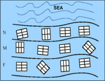
The experiment was set up as follows: A beach on the Otago Peninsula was divided into 3 areas (near, middle, and far) according to the distance from the sea. Within each of these three areas 4 quadrats were randomly chosen, and then each site was divided into 6 equal plots. Each plot within each quadrat was allocated to 1 of 6 groups of harvesters (6 groups who collected the data), resulting in each group harvesting one plot in every quadrat for every area.
The diagram below illustrates this layout:
0. Read and Format the data
0a. Read in the data
First check you have installed the package readxl (see Section 2.6) and set the working directory (see Section 2.1), using instructions in Getting started with R.
Load the data into R.
We can then view the first 6 lines of the cockles data. This is a tibble (simplified data frame) containing data from a study investigating cockle biomass and density in relation to distance from sea water.
Code
#load readxl package
library(readxl)

#load the .xls data file using read_xls()
#name this data cockles
cockles<-read_xls("Cockle Data.xls")

#by default head() displays the first 6 lines of the data frame.
#can change the number of lines using the argument n=
head(cockles)
Code
#load readxl package
library(readxl)
Warning: package 'readxl' was built under R version 4.2.2Code
#load the .xls data file using read_xls()
#name this data cockles
cockles<-read_xls("Cockle Data.xls")

#by default head() displays the first 6 lines of the data frame.
#can change the number of lines using the argument n=
head(cockles)
# A tibble: 6 × 6
Area Quadrat Group Biomass `Cockle No (Density)` `Water level`
<chr> <dbl> <dbl> <dbl> <dbl> <dbl>
1 N 1 2 3.05 68 1
2 N 2 2 3.29 104 0
3 N 3 2 4.29 146 3
4 N 4 2 4.64 124 15
5 M 1 2 2.42 127 39
6 M 2 2 1.89 121 39The data frame contains the following variables: Area (distance from the channel; N=near, M=middle, F=far), Quadrat (sampling unit), Group (group of harvesters), Water level (standardized value giving height relative to water table), Biomass (weight in kgs), and Cockle No (Density) (number of cockles found).
0b. Format the data
R has classified Area as a character variable, but it is actually a factor with 3 levels (N=near, M=middle, and F=far).
Reassign Area and Group as factor variables. Rename the Cockle No (Density) and Water level variables (without spaces, shorter names) for easier reference later.
Check your new data frame.
Code
#recode Area as a factor variable
cockles$Area<-as.factor(cockles$Area)

#columns 1-4 keep the same variable names, overwrite columns 5 and 6
colnames(cockles)<-c("Area","Quadrat","Group","Biomass","Density","Wlevel")
Code
#recode Area as a factor variable
cockles$Area<-as.factor(cockles$Area)

#recode Group as a factor variable
cockles$Group<-as.factor(cockles$Group)

#columns 1-4 keep the same variable names, overwrite columns 5 and 6
colnames(cockles)<-c("Area","Quadrat","Group","Biomass","Density","Wlevel")

head(cockles)
# A tibble: 6 × 6
Area Quadrat Group Biomass Density Wlevel
<fct> <dbl> <fct> <dbl> <dbl> <dbl>
1 N 1 2 3.05 68 1
2 N 2 2 3.29 104 0
3 N 3 2 4.29 146 3
4 N 4 2 4.64 124 15
5 M 1 2 2.42 127 39
6 M 2 2 1.89 121 391. Box Plot, Histograms, Confidence Intervals (single predictor)
1a. Box Plot
First we want a visual representation of our data.
Draw the box and whisker plots for Biomass by Area for the three locations (F, M, and N).
Describe what you can see from this plot, and state any tentative conclusions that you make.
Code
#boxplot() function uses the formula y~x.
#since we are interested in how area affects biomass, our x (explanatory) variable is Area, our y (Response) variable is Biomass.
boxplot(cockles$Biomass~cockles$Area)
Code
#boxplot() function uses the formula y~x.
#since we are interested in how area affects biomass, our x (explanatory) variable is Area, our y (Response) variable is Biomass.
boxplot(cockles$Biomass~cockles$Area) 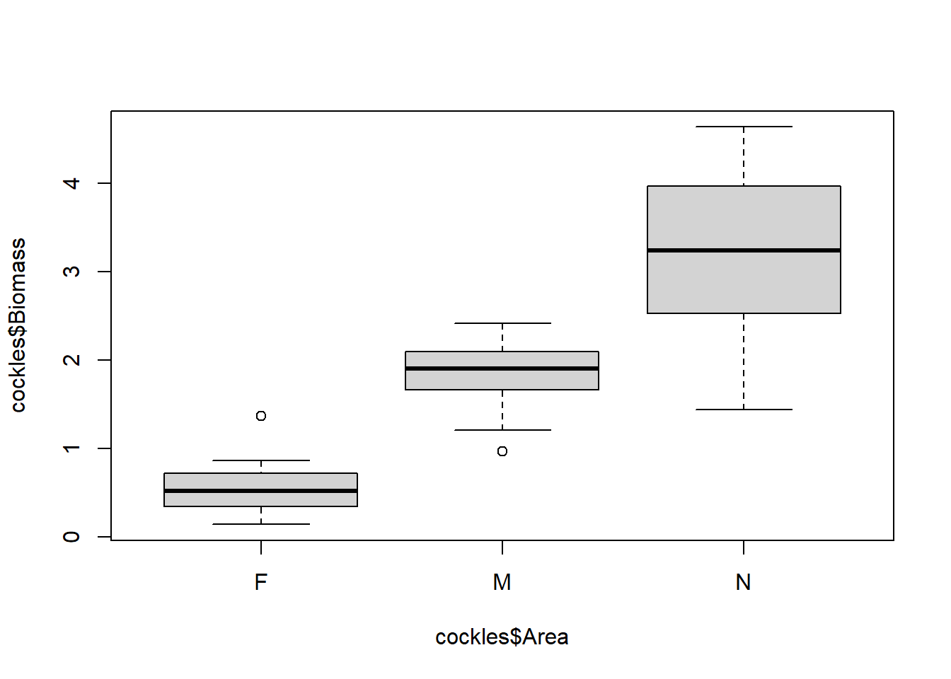
On a box plot the thick black line indicates the median, with the lower quartile (25% of values are less than this) and upper quartile (75% of values are less than this) enclosing the grey box (middle 50% of values). The minimum and maximum are shown by horizontal lines below and above this box. Outliers are indicates with points.
There is considerable variation in biomass by area, shown by the differing medians and limited overlap between the middle 50% of values. Cockles in the near area have the largest biomass measurements and the most variability. Those in the far area have the smallest biomass, and variability is similar to that of the middle area. There is strong indication of a significant difference between the median biomass for middle and far areas, as there is no overlap except for outliers.
1b. Histograms
Draw the histograms of Biomass for each of the three Areas.
To do this, we must subset the observations by Area when creating the graph.
Code
#use the hist() function to produce a histogram.
#the use of [] brackets to subset the Area variable indicates that we only want the Biomass measurements corresponding to cockles in the near (N) Area.
hist(cockles$Biomass[cockles$Area=="N"])
Repeat and modify the above code for the Areas ‘middle’ and ‘far’ and comment on your results.
Code
#use the hist() function to produce a histogram.
#the use of [] brackets to subset the Area variable indicates that we only want the Biomass measurements corresponding to cockles in the near (N) Area.
hist(cockles$Biomass[cockles$Area=="N"]) 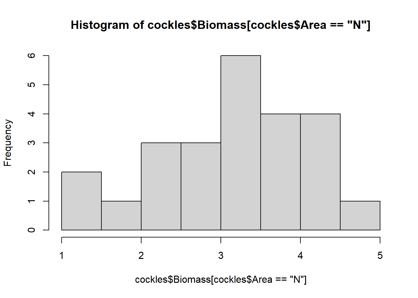
Code
hist(cockles$Biomass[cockles$Area=="M"]) 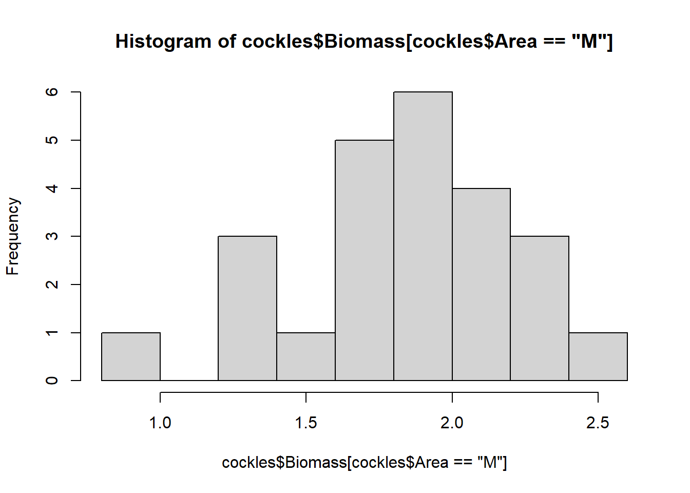
Code
hist(cockles$Biomass[cockles$Area=="F"]) 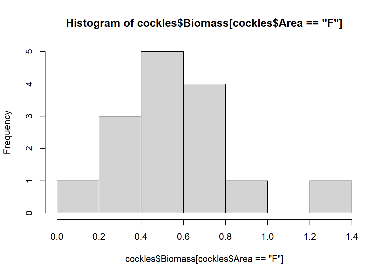
The biomass for all areas are roughly normally distributed around their varying modes (most common values), although they show some skew. The near and middle areas are left skewed, while the far area is right skewed.
1c. Confidence Intervals by hand
Construct 95% confidence intervals for the three mean Biomass levels.
A 95% confidence interval for the mean of normally distributed data can be calculated by hand using the following formula
\[ \overline{x} \pm 1.96 * \frac{\sigma_x}{\sqrt{n}}\] What do you conclude from your confidence intervals?
We need to calculate the components \(\overline{x}\) (estimate of mean), and \(\frac{\sigma_x}{\sqrt{n}}\) (estimate of standard error of the mean).
Code
#mean() function to calculate the mean biomass for near cockles
mean(cockles$Biomass[cockles$Area=="N"])

#sd() function to calculate the standard deviation
#length() to calculate the number of observations
#sqrt() to take the square root.
#together these compute the estimate of the standard error of the mean biomass for near cockles
sd(cockles$Biomass[cockles$Area=="N"])/sqrt(length(cockles$Biomass[cockles$Area=="N"]))
These values can be substituted into the formula to construct a 95% confidence interval for the mean Biomass of near cockles.
Repeat the procedure for the middle and far subsets of cockles.
Code
#mean() function to calculate the mean biomass for near cockles
nm<-mean(cockles$Biomass[cockles$Area=="N"])

#sd() function to calculate the standard deviation
#length() to calculate the number of observations
#sqrt() to take the square root.
#together these compute the estimate of the standard error of the mean biomass for near cockles
nse<-sd(cockles$Biomass[cockles$Area=="N"])/sqrt(length(cockles$Biomass[cockles$Area=="N"]))
near.lower<-nm-(1.96*nse)
near.upper<-nm+(1.96*nse)


mm<-mean(cockles$Biomass[cockles$Area=="M"])

mse<-sd(cockles$Biomass[cockles$Area=="M"])/sqrt(length(cockles$Biomass[cockles$Area=="M"]))

middle.lower<-mm-(1.96*mse)
middle.upper<-mm+(1.96*mse)


fm<-mean(cockles$Biomass[cockles$Area=="F"])

fse<-sd(cockles$Biomass[cockles$Area=="F"])/sqrt(length(cockles$Biomass[cockles$Area=="F"]))
far.lower<-fm-(1.96*fse)
far.upper<-fm+(1.96*fse)


print(c(near.lower,near.upper,middle.lower,middle.upper,far.lower,far.upper))
[1] 2.8342583 3.5515750 1.6855493 1.9886174 0.4029955 0.7236712We can be 95% confident that the true mean biomass for the near area lies between 2.8342583 and 3.5515750 kgs, between 1.6855493 and 1.9886174 kgs for the middle area, and between 0.4029955 and 0.7236712 kgs for the far area. As there is no overlap in these confidence intervals there is significant evidences of a difference in means between the areas.
1d. Confidence Intervals in R
Construct 95% confidence intervals for the three mean Biomass levels using R.
The t.test() function for one sample will calculate these.
Code
t.test(cockles$Biomass[cockles$Area=="N"])You can find the limits under \(\verb!95 percent confidence interval:!\) in the output. The confidence interval resulting from this test will be slightly wider than the one you found by hand. It uses the t-distribution to calculate the multiplier (instead of the default value 1.96), which is best practice when we do not know the population standard deviation.
Repeat the procedure for the middle and far subsets of cockles.
Code
t.test(cockles$Biomass[cockles$Area=="N"])
    One Sample t-test

data:  cockles$Biomass[cockles$Area == "N"]
t = 17.449, df = 23, p-value = 9.257e-15
alternative hypothesis: true mean is not equal to 0
95 percent confidence interval:
 2.814375 3.571458
sample estimates:
mean of x
 3.192917
Code
t.test(cockles$Biomass[cockles$Area=="M"])
    One Sample t-test

data:  cockles$Biomass[cockles$Area == "M"]
t = 23.762, df = 23, p-value < 2.2e-16
alternative hypothesis: true mean is not equal to 0
95 percent confidence interval:
 1.677149 1.997018
sample estimates:
mean of x
 1.837083
Code
t.test(cockles$Biomass[cockles$Area=="F"])
    One Sample t-test

data:  cockles$Biomass[cockles$Area == "F"]
t = 6.8863, df = 14, p-value = 7.486e-06
alternative hypothesis: true mean is not equal to 0
95 percent confidence interval:
 0.3878790 0.7387877
sample estimates:
mean of x
0.5633333
Slightly different confidence limits, but come to the same conclusions as those calculated by hand.
2. Box Plot, Confidence Intervals (multiple predictors)
2a. Box Plot
Construct box and whisker plots for the Density per Quadrat for the three Areas.
What are some features of this graph that stand out? What is the extra point that you see for 2.M and how may it affect your data?
Code
#include each quadrat and area combination by multiplying the quadrat and area variables,to form the explanatory levels
boxplot(cockles$Density ~ cockles$Quadrat*cockles$Area)
Code
#include each quadrat and area combination by multiplying the quadrat and area variables,to form the explanatory levels
boxplot(cockles$Density ~ cockles$Quadrat*cockles$Area) 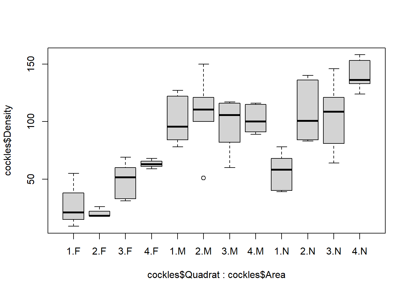
There is limited variation in density by quadrat for the middle area, the middle 50% of values are all overlapping and medians are very close together. Much more variation between quadrats for the far and near areas. For the 2nd quadrat of the far area the median, lower quartile and minimum are equivalent, suggesting there may only a few observations.
The extra point for 2.M (2nd quadrat in the middle area) has been distinguished as an outlier by R, due to the difference between this density (around 50) and the other observed densities (between 100 and 150). It may affect the data by dragging down the mean density for the middle area and exerting more influence on estimates than other points.
2b. Confidence Intervals in R
Construct the 95% confidence intervals for the mean Density at N, M and F for each of the Quadrats.
Report your conclusions from the confidence intervals for all Area and Quadrat combinations.
This code calculates the lower and upper limits of a 95% confidence interval for cockle Density in the first of the near Quadrats.
Code
#note how we must specify both the Area and (&) Quadrat to subset Density by
t.test(cockles$Density[cockles$Area=="N"&cockles$Quadrat=="1"])
Code
#note how we must specify both the Area and (&) Quadrat to subset Density by
t.test(cockles$Density[cockles$Area=="N"&cockles$Quadrat=="1"])
    One Sample t-test

data:  cockles$Density[cockles$Area == "N" & cockles$Quadrat == "1"]
t = 8.8873, df = 5, p-value = 0.0003001
alternative hypothesis: true mean is not equal to 0
95 percent confidence interval:
 40.39478 73.27189
sample estimates:
mean of x
 56.83333
Code
#note how we must specify both the Area and (&) Quadrat to subset Density by
t.test(cockles$Density[cockles$Area=="N"&cockles$Quadrat=="2"])
    One Sample t-test

data:  cockles$Density[cockles$Area == "N" & cockles$Quadrat == "2"]
t = 10.486, df = 5, p-value = 0.0001361
alternative hypothesis: true mean is not equal to 0
95 percent confidence interval:
  81.0206 133.6461
sample estimates:
mean of x
 107.3333
Code
#note how we must specify both the Area and (&) Quadrat to subset Density by
t.test(cockles$Density[cockles$Area=="N"&cockles$Quadrat=="3"])
    One Sample t-test

data:  cockles$Density[cockles$Area == "N" & cockles$Quadrat == "3"]
t = 8.7986, df = 5, p-value = 0.0003147
alternative hypothesis: true mean is not equal to 0
95 percent confidence interval:
  74.20551 135.46116
sample estimates:
mean of x
 104.8333
Code
#note how we must specify both the Area and (&) Quadrat to subset Density by
t.test(cockles$Density[cockles$Area=="N"&cockles$Quadrat=="4"])
    One Sample t-test

data:  cockles$Density[cockles$Area == "N" & cockles$Quadrat == "4"]
t = 26.489, df = 5, p-value = 1.433e-06
alternative hypothesis: true mean is not equal to 0
95 percent confidence interval:
 126.414 153.586
sample estimates:
mean of x
140 3. Simple Linear Regression, ANOVA, Hypothesis Test
3a. Simple Linear Regression and ANOVA
Fit a linear model with Biomass as the response and Area as the predictor.
Carry out the accompanying one-factor Analysis of Variance (ANOVA) and report your findings from the ANOVA.
Code
#fit a linear model using lm() and the format response~explanatory (as for the box plot)
cockles.ba<-lm(cockles$Biomass~cockles$Area)

#output model summary
summary(cockles.ba)

#anova() calculates the ANOVA object from a fitted model
anova(cockles.ba)
Code
#fit a linear model using lm() and the format response~explanatory (as for the box plot)
cockles.ba<-lm(cockles$Biomass~cockles$Area)

#output model summary
summary(cockles.ba)
Call:
lm(formula = cockles$Biomass ~ cockles$Area)

Residuals:
     Min       1Q   Median       3Q      Max
-1.75292 -0.32333  0.03667  0.28500  1.44708

Coefficients:
              Estimate Std. Error t value Pr(>|t|)
(Intercept)     0.5633     0.1605   3.510 0.000858 ***
cockles$AreaM   1.2737     0.2046   6.225 5.15e-08 ***
cockles$AreaN   2.6296     0.2046  12.851  < 2e-16 ***
---
Signif. codes:  0 '***' 0.001 '**' 0.01 '*' 0.05 '.' 0.1 ' ' 1

Residual standard error: 0.6217 on 60 degrees of freedom
Multiple R-squared:  0.7388,    Adjusted R-squared:  0.7301
F-statistic: 84.86 on 2 and 60 DF,  p-value: < 2.2e-16
Code
#anova() calculates the ANOVA object from a fitted model
anova(cockles.ba)
Analysis of Variance Table
Response: cockles$Biomass
Df Sum Sq Mean Sq F value Pr(>F)
cockles$Area 2 65.591 32.795 84.858 < 2.2e-16 ***
Residuals 60 23.189 0.386
---
Signif. codes: 0 '***' 0.001 '**' 0.01 '*' 0.05 '.' 0.1 ' ' 1The ANOVA returned p-value of <2.2 e-16 for the area variable, indicating a significant decrease in variance explained if this is removed from the model. A p-value of 0.05 or less is typically used as the cut-off for determining significance.
This can be translated to an indication that the model for cockle biomass is significantly improved with the inclusion of the area variable.
Looking at the parameter estimates in the summary of the linear model we see that compared to the baseline far area, biomass in the middle area is an average of 1.2737 kgs greater and biomass in the near area 2.6296 kgs greater.
3b. Hypothesis Test
Carry out one independent samples test (hypothesis test) for one pair of the means.
You may have noticed when using t.test() earlier that there is extra information in the output in addition to the confidence interval. This function also performs hypothesis tests. When you provide it with a single vector of data it tests against the null hypothesis that the mean of that data is equal to 0. When you provide it with two vectors of data it tests against the null hypothesis that the difference in means is equal to 0.
Report your conclusions from this independent samples t-test.
Code
#test if variances for Biomass are equal between the two Areas using the var.test() function.
#alternative="two-sided" indicates that we are interested in differences between the variances in any direction.
var.test(cockles$Biomass[cockles$Area=="N"],cockles$Biomass[cockles$Area=="M"],
         alternative = "two.sided")
If the variance test output p-value is less than 0.05 this indicates significant evidence against null hypothesis that variances are equal, and we should use var.equal=FALSE in the t test.
If the p-value is greater than 0.05 we should use var.equal=TRUE in the t test.
Code
#compare the Biomass for near and middle Areas.
#paired=FALSE indicates independent samples (as specified in the question).
t.test(cockles$Biomass[cockles$Area=="N"],cockles$Biomass[cockles$Area=="M"],paired=FALSE)
Code
#test if variances for Biomass are equal between the two Areas using the var.test() function.
#alternative="two-sided" indicates that we are interested in differences between the variances in any direction.
var.test(cockles$Biomass[cockles$Area=="N"],cockles$Biomass[cockles$Area=="M"],
         alternative = "two.sided")
    F test to compare two variances

data:  cockles$Biomass[cockles$Area == "N"] and cockles$Biomass[cockles$Area == "M"]
F = 5.602, num df = 23, denom df = 23, p-value = 0.000108
alternative hypothesis: true ratio of variances is not equal to 1
95 percent confidence interval:
  2.423377 12.949755
sample estimates:
ratio of variances
          5.601976
Code
#compare the Biomass for near and middle Areas.
#paired=FALSE indicates independent samples (as specified in the question).
#var.equal=F indicates the variances are not equal, as tested using var.test().
t.test(cockles$Biomass[cockles$Area=="N"],cockles$Biomass[cockles$Area=="M"],paired=FALSE,
       var.equal=F)
    Welch Two Sample t-test

data:  cockles$Biomass[cockles$Area == "N"] and cockles$Biomass[cockles$Area == "M"]
t = 6.8252, df = 30.958, p-value = 1.21e-07
alternative hypothesis: true difference in means is not equal to 0
95 percent confidence interval:
 0.9506591 1.7610075
sample estimates:
mean of x mean of y
 3.192917  1.837083
If a hypothesis test returns a p-value of <0.05 this indicates significant evidence against the null hypothesis.
When comparing the biomass in the near and middle areas the null hypothesis is that there is no true difference in means, while the alternative is that there is a true difference in means. The p-value for the test is 1.21e-07, giving us significant evidence to reject the null hypothesis in favour of the alternative and conclude there is a difference in mean biomass between the near and middle areas.
The associated 95% confidence interval for the difference in means shows that mean cockle biomass is estimated to be between 2.4234 and 12.9498 kgs greater in the near area than the middle area. Note: the order of differing corresponds to first variable - second variable in the t.test() function.
4. Multiple Linear Regression, ANOVA, Interaction and Residual Plots
4a. Multiple Linear Regression and ANOVA
A limitation of our previous analysis is that we were only able to consider one predictor variable at a time. A method that allows us to consider several of these variables simultaneously is multiple regression.
Add the Group variable to the linear model, making sure you also include an interaction between Area and Group.
Then carry out a two-factor Analysis of Variance (ANOVA) for this fitted model.
Report your findings and compare with the one-factor ANOVA results from Task 3a.
Code
#same procedure as 3a, with addition of interaction between Area and Group
cockles.bga<-lm(cockles$Biomass~cockles$Area*cockles$Group)

#output model summary
summary(cockles.bga)

#calculate ANOVA object
anova(cockles.bga)
Code
#same procedure as 3a, with addition of interaction between Area and Group
cockles.bga<-lm(cockles$Biomass~cockles$Area*cockles$Group)

#output model summary
summary(cockles.bga)
Call:
lm(formula = cockles$Biomass ~ cockles$Area * cockles$Group)

Residuals:
    Min      1Q  Median      3Q     Max
-1.5225 -0.2850  0.0275  0.2888  1.4875

Coefficients:
                             Estimate Std. Error t value Pr(>|t|)
(Intercept)                   0.61500    0.45914   1.339 0.187146
cockles$AreaM                 1.01250    0.56233   1.801 0.078479 .
cockles$AreaN                 2.34750    0.56233   4.175 0.000135 ***
cockles$Group2                0.07000    0.64932   0.108 0.914630
cockles$Group3               -0.05500    0.64932  -0.085 0.932873
cockles$Group4               -0.37500    0.64932  -0.578 0.566463
cockles$Group5               -0.05000    0.56233  -0.089 0.929543
cockles$Group6                0.04833    0.59275   0.082 0.935373
cockles$AreaM:cockles$Group2  0.20000    0.79525   0.251 0.802578
cockles$AreaN:cockles$Group2  0.78500    0.79525   0.987 0.328868
cockles$AreaM:cockles$Group3  0.38000    0.79525   0.478 0.635080
cockles$AreaN:cockles$Group3  0.15250    0.79525   0.192 0.848791
cockles$AreaM:cockles$Group4  0.28750    0.79525   0.362 0.719403
cockles$AreaN:cockles$Group4  0.10500    0.79525   0.132 0.895546
cockles$AreaM:cockles$Group5  0.46000    0.72596   0.634 0.529523
cockles$AreaN:cockles$Group5  0.26000    0.72596   0.358 0.721910
cockles$AreaM:cockles$Group6  0.29167    0.74977   0.389 0.699105
cockles$AreaN:cockles$Group6  0.44167    0.74977   0.589 0.558761
---
Signif. codes:  0 '***' 0.001 '**' 0.01 '*' 0.05 '.' 0.1 ' ' 1

Residual standard error: 0.6493 on 45 degrees of freedom
Multiple R-squared:  0.7863,    Adjusted R-squared:  0.7056
F-statistic: 9.739 on 17 and 45 DF,  p-value: 5.294e-10
Code
#calculate ANOVA object
anova(cockles.bga)
Analysis of Variance Table
Response: cockles$Biomass
Df Sum Sq Mean Sq F value Pr(>F)
cockles$Area 2 65.591 32.795 77.7847 2.491e-15 ***
cockles$Group 5 3.000 0.600 1.4233 0.2343
cockles$Area:cockles$Group 10 1.215 0.122 0.2883 0.9806
Residuals 45 18.973 0.422
---
Signif. codes: 0 '***' 0.001 '**' 0.01 '*' 0.05 '.' 0.1 ' ' 1The ANOVA returned p-value of <2.491 e-15 for the area variable, indicating a significant decrease in the variance explained if this is removed from the model. The group variable has a p-value of 0.2343, and the area:group interaction is 0.9806.
This can be translated to an indication that the model for cockle biomass is significantly improved with the inclusion of the area variable, but the inclusion of group and an area:group interaction is unnecessary.
To avoid over fitting these variables should be removed from the model, and interpretation should focus on the simple linear regression with the area variable alone (Task 3a.)
If we were to interpret the coefficients of this full model this is what we would find - with all other variables held constant, biomass in the middle area is an average of 1.01250 kgs greater (non-significant) and biomass in the near area 2.34750 kgs greater (significant) than the baseline mean biomass in the far area.
Cockles in group 2 and 6 have a slightly higher mean biomass than those in group 1, while those in groups 3, 4 and 5 have a lower mean biomass. These effects are all non-significant however.
Compared to the baseline group 1, being in any other group also increased the estimated positive effect on biomass of being in the middle or near areas, but these interactions were not significant.
4b. Residual Plots for Fitted Models
An important part of model fitting is checking that the model assumptions have been met and there is no significant lack of fit.
Obtain the mean interaction plots and the residual plots for the model in Task 4a..
Discuss what these graphs tell us about the fitted model.
Code
#interaction.plot() function generates an interaction plot.
#first variable specifies the predictor on the x axis
#second variable specifies the trace predictor (the plot will show a line describing the relationship between the x and y variables for each level of this variable)
#third variable is the response on the y axis.
interaction.plot(cockles$Group,cockles$Area,cockles$Biomass,fun=mean)
The interaction plot shows how the relationship between the group and biomass variables changes according to area. If these lines cross it is an indication an interaction term should be included in the model.
Code
#calling plot() on a fitted model object will automatically generate the relevant residual plots
plot(cockles.bga)
In the first residual scatter plot, we need to check that the residuals are randomly scattered around the mean of 0 (linear relationship between variables), and there is no systematic pattern in the spread of the residuals across the fitted values (constant variance) when excluding outliers.
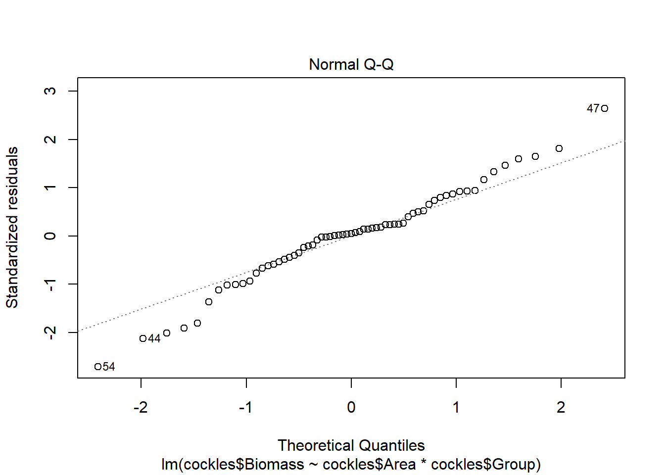
In the second plot we check that the points follow the standard normal quantile line (residuals are standard normally distributed).
The third plot can be used to check the spread of standardised residuals, these should fall between -2 and +2. This corresponds to <1.4 when the square root is taken.
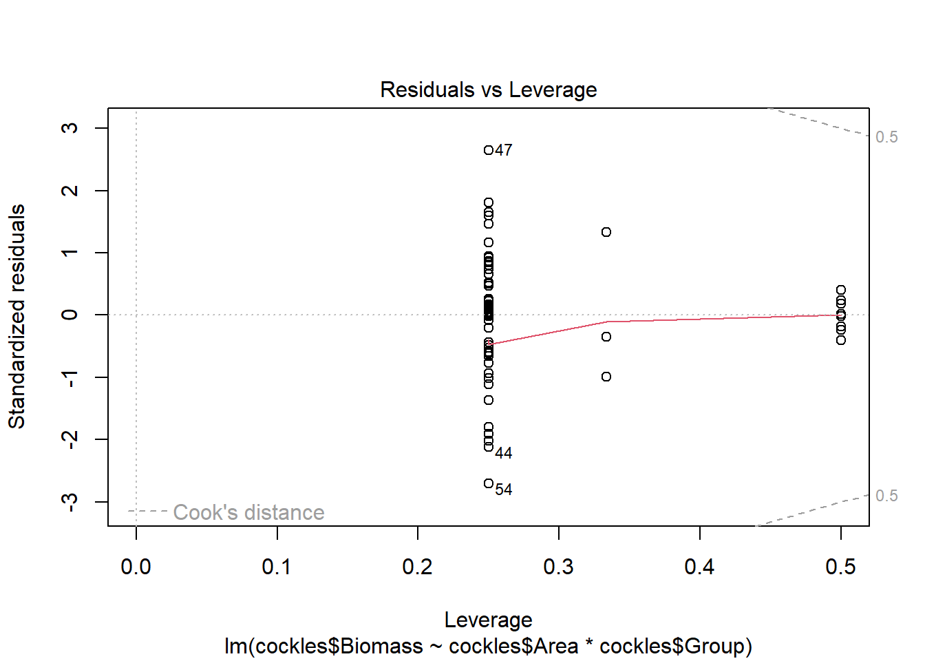
The fourth plot shows the influence of each observation on parameter estimates, with highly influential points automatically labelled. Influence is due to a combination of leverage and the value of standardised residuals. Leverage is a measure of how much an observation affects the fitted line (due to its position in the data set) and the standardised residual value indicates the extent to which the observation is an outlier. Points with high influence potentially require further investigation.
If any of the above assumptions are not met, it indicates that there is a problem with the estimated regression equation. Although there are ways to solve such problems, they are beyond Year 13 level. You can learn these and a lot more about advanced regression methods at university, typically in a second year Statistics course.
Code
#interaction.plot() function generates an interaction plot.
#first variable specifies the predictor on the x axis
#second variable specifies the trace predictor (the plot will show a line describing the relationship between the x and y variables for each level of this variable)
#third variable is the response on the y axis.
interaction.plot(cockles$Group,cockles$Area,cockles$Biomass,fun=mean) 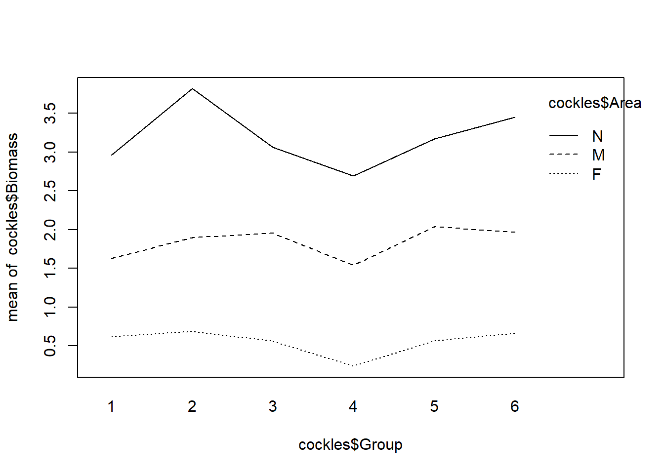
This plot shows there is a clear difference in mean biomass by area, as the lines representing levels of area are well separated. There is no evidence of an interaction with the group variable, the lines are parallel which suggests the relationship between area and biomass does not change much according to group.
Code
#calling plot() on a fitted model object will automatically generate the relevant residual plots
plot(cockles.bga) 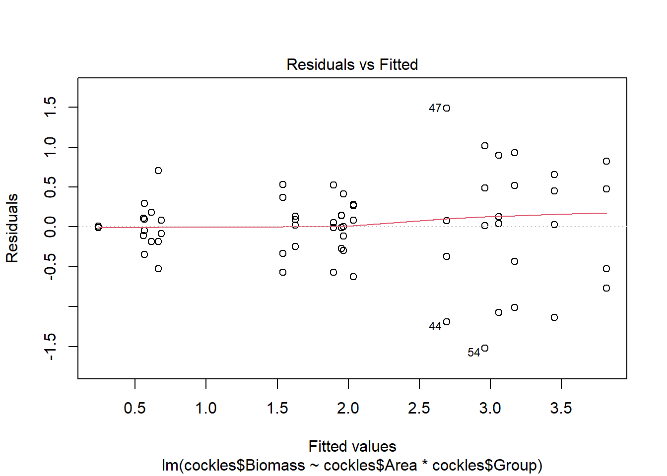
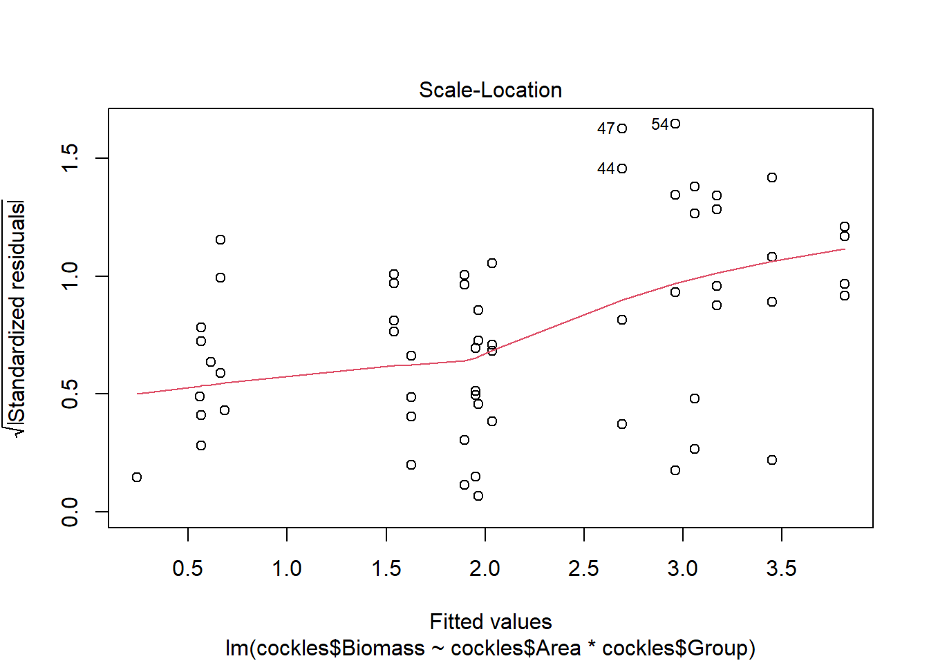
The residuals show evidence of non-constant variance, for larger fitted values (on the right hand side of the plot) there is much more variation. If we imagine horizontal lines (top and bottom) around the largest residuals (excluding outliers) these would fan out moving from left to right.
There are a few outliers with square root standardised residuals around 1.5 (corresponding to 2.25 when squared).
The normal qq plot looks ok, the standardised residuals are fairly close to the standard normal quantiles. There is some separation at the more extreme quantiles but this is typically expected.
The fourth plot indicates a couple of highly influential points - observations 44, 47 and 54. None of these points have particularly high leverage, instead their influence is due to large standardised residual values (they are outliers). This may be due to measurement or transcription errors, however their values are not dramatically different from the other observations. It is more likely that there is additional natural variation that has not been accounted for by our model.
5. Practice: Simple Linear Regression, ANOVA
5a. Scatter Plot
Graph Biomass against Density as a scatter plot, with Biomass as the response and Density as the predictor.
What pattern can you see in the scatter plot?
Code
#the plot() function generates a scatter plot when both variables are continuous.
#first argument is the x (explanatory) variable
#second is the y (response) variable.
plot(cockles$Density,cockles$Biomass)
Code
#the plot() function generates a scatter plot when both variables are continuous.
#first argument is the x (explanatory) variable
#second is the y (response) variable.
plot(cockles$Density,cockles$Biomass) 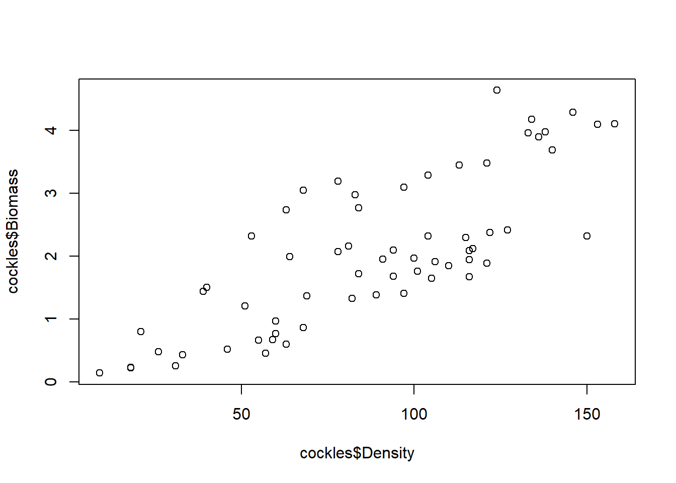
Moderately strong, positive linear relationship. As density increases, so does biomass.
5b. Linear Regression and ANOVA
Fit a linear regression, with Biomass as the response variate and Density as the explanatory variate.
Remember to check the residual plots.
Write out the model, and report your findings from this linear regression.
This code has been hidden initially, so you can try to modify code from Task 3a ( which fits a linear regression and calculates the ANOVA object for a similar model).
You can then reveal the code and check your results.
Code
cockle.bd<-lm(cockles$Biomass~cockles$Density)
summary(cockle.bd)
anova(cockle.bd)

plot(cockle.bd)
Code
cockle.bd<-lm(cockles$Biomass~cockles$Density)
summary(cockle.bd)
Call:
lm(formula = cockles$Biomass ~ cockles$Density)

Residuals:
    Min      1Q  Median      3Q     Max
-1.2964 -0.6085 -0.1389  0.6263  1.6778

Coefficients:
                 Estimate Std. Error t value Pr(>|t|)
(Intercept)     -0.158045   0.235560  -0.671    0.505
cockles$Density  0.025163   0.002469  10.193 8.55e-15 ***
---
Signif. codes:  0 '***' 0.001 '**' 0.01 '*' 0.05 '.' 0.1 ' ' 1

Residual standard error: 0.7338 on 61 degrees of freedom
Multiple R-squared:  0.6301,    Adjusted R-squared:  0.624
F-statistic: 103.9 on 1 and 61 DF,  p-value: 8.549e-15
Code
anova(cockle.bd) Analysis of Variance Table
Response: cockles$Biomass
Df Sum Sq Mean Sq F value Pr(>F)
cockles$Density 1 55.936 55.936 103.89 8.549e-15 ***
Residuals 61 32.843 0.538
---
Signif. codes: 0 '***' 0.001 '**' 0.01 '*' 0.05 '.' 0.1 ' ' 1The ANOVA returned p-value of 8.549 e-15 for the density variable, indicating a significant decrease in the variance explained if this is removed from the model. This indicates that the model for cockle biomass is significantly improved with the inclusion of the density variable.
The fitted model can be written as follows
\[BIOMASS = -0.1581 + 0.0252_{DENSITY}\] For each one unit increase in density, mean cockle biomass increases by 0.0252 kgs.
Code
plot(cockle.bd)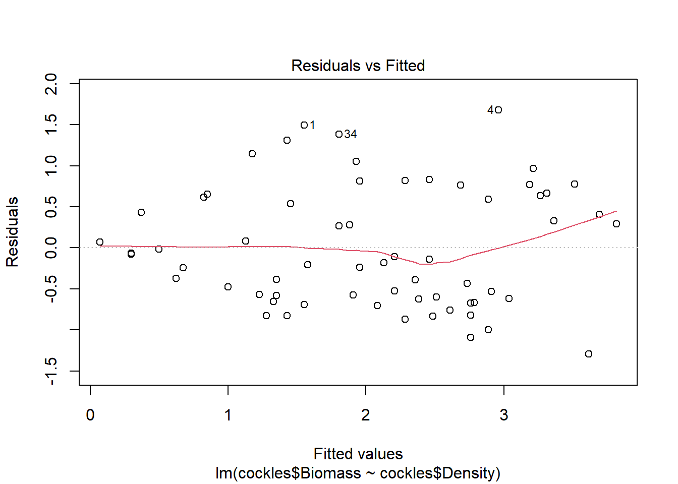
The residuals show fairly constant variance, and there are no points with residual values greater than \(\pm 2\). There is some suggestion of non-linearity in the relationship for larger fitted values (indicated by the red line which deviates from 0 on the right side of the plot), although this is not major.
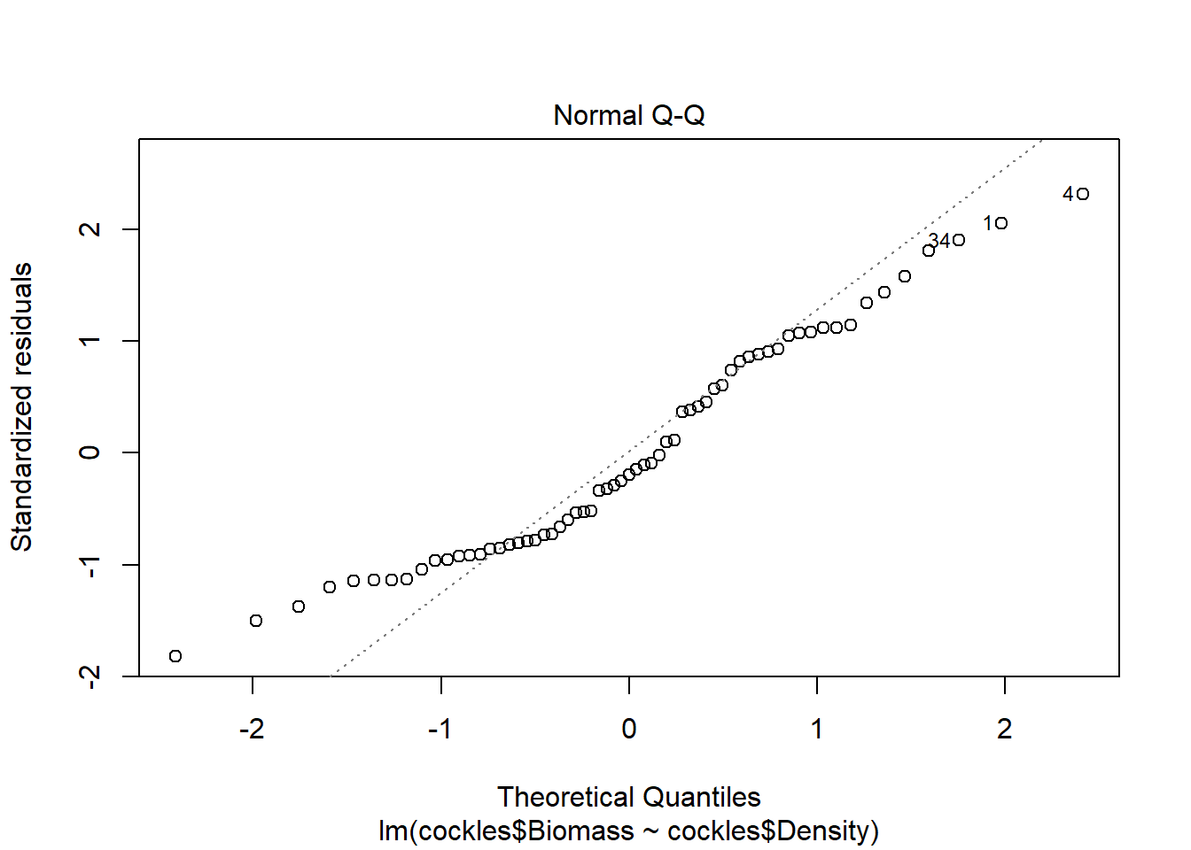
The normal qq plot looks ok, the standardised residuals are fairly close to the standard normal quantiles. There is some separation at the more extreme quantiles but this is typically expected.
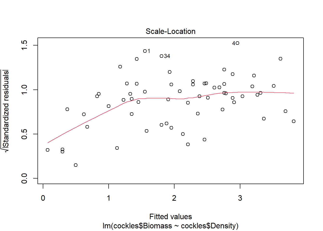
There are a few outliers with square root standardised residuals around 1.5 (corresponding to 2.25 when squared).
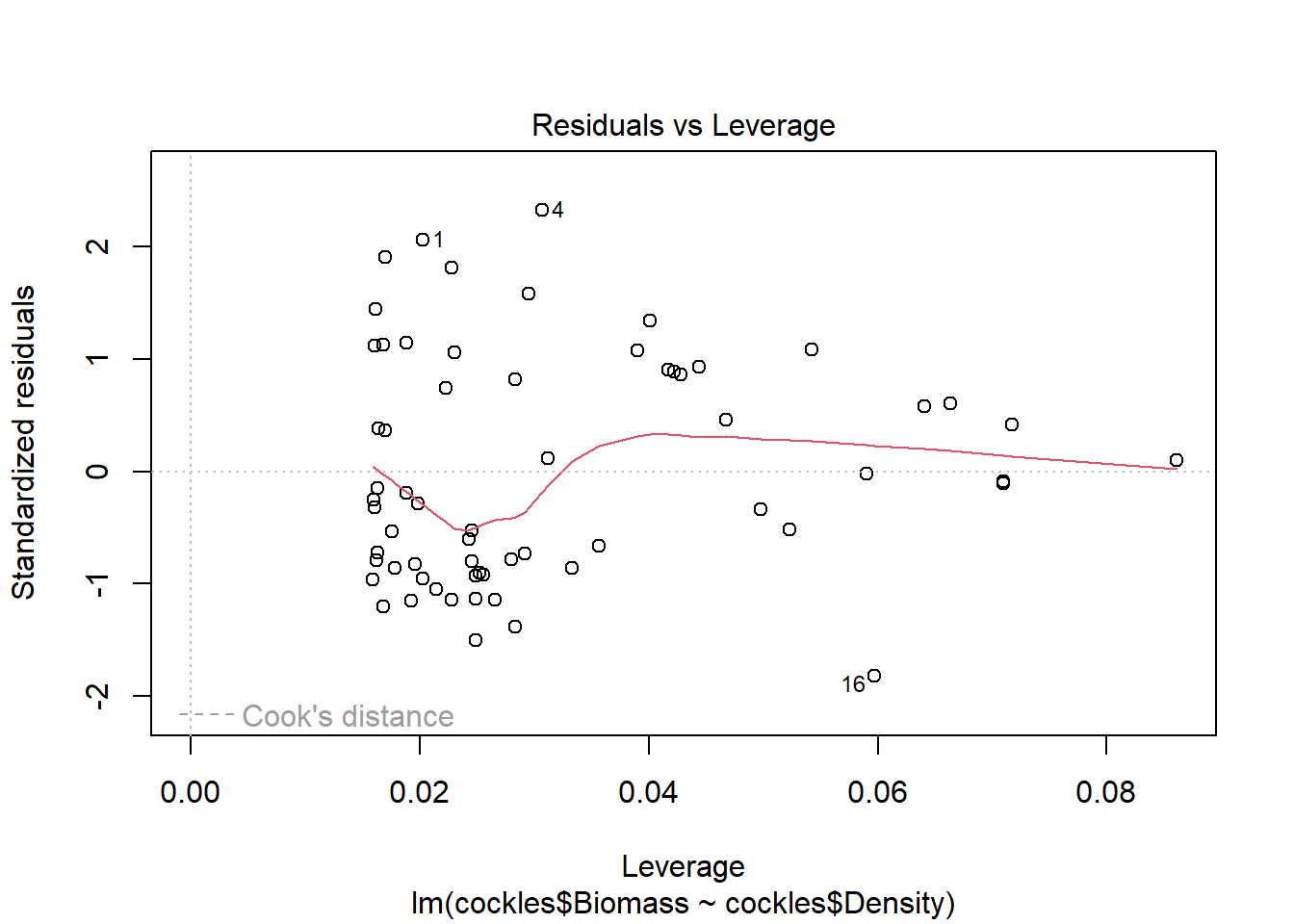
The fourth plot indicates a couple of highly influential points - observations 1, 4 and 16. The influence of points 1 and 4 is due to large standardised residual values (they are outliers). This may be due to measurement or transcription errors, however their values are not dramatically different from the other observations. It is more likely that there is additional natural variation that has not been accounted for by our model. Observation 16 has quite a large negative residual value, and is also in a position of high leverage within the data set. It is likely the most influential observation.
6. Practice: Multiple Linear Regression, ANOVA
Carry out a multiple regression, with Biomass as the response, and Density and Wlevel as the predictors. Make sure to include the interaction between Density and Wlevel.
Check the residual plots to assess your model.
Write out the model, and report your findings from this linear regression.
This code has again been hidden initially, so you can try to modify code from Task 4 ( which fits a linear regression and calculates the ANOVA object for a similar interaction model).
You can then reveal the code and check your results.
Code
cockles.bdw<-lm(cockles$Biomass~cockles$Density*cockles$Wlevel)
summary(cockles.bdw)
anova(cockles.bdw)

plot(cockles.bdw)
Code
cockles.bdw<-lm(cockles$Biomass~cockles$Density*cockles$Wlevel)
summary(cockles.bdw)
Call:
lm(formula = cockles$Biomass ~ cockles$Density * cockles$Wlevel)

Residuals:
     Min       1Q   Median       3Q      Max
-0.97220 -0.21538 -0.05472  0.12870  1.34759

Coefficients:
                                 Estimate Std. Error t value Pr(>|t|)
(Intercept)                     7.169e-01  2.366e-01   3.031 0.003619 **
cockles$Density                 2.583e-02  2.341e-03  11.034 5.66e-16 ***
cockles$Wlevel                 -1.243e-02  5.415e-03  -2.295 0.025317 *
cockles$Density:cockles$Wlevel -2.373e-04  6.232e-05  -3.807 0.000337 ***
---
Signif. codes:  0 '***' 0.001 '**' 0.01 '*' 0.05 '.' 0.1 ' ' 1

Residual standard error: 0.3629 on 59 degrees of freedom
Multiple R-squared:  0.9125,    Adjusted R-squared:  0.908
F-statistic:   205 on 3 and 59 DF,  p-value: < 2.2e-16
Code
anova(cockles.bdw)Analysis of Variance Table
Response: cockles$Biomass
Df Sum Sq Mean Sq F value Pr(>F)
cockles$Density 1 55.936 55.936 424.623 < 2.2e-16 ***
cockles$Wlevel 1 23.161 23.161 175.823 < 2.2e-16 ***
cockles$Density:cockles$Wlevel 1 1.910 1.910 14.496 0.0003366 ***
Residuals 59 7.772 0.132
---
Signif. codes: 0 '***' 0.001 '**' 0.01 '*' 0.05 '.' 0.1 ' ' 1The ANOVA returned p-values of <2.2 e-16 for the density and water level variables along with 0.0003 for their interaction, indicating a significant decrease in variance explained if any are removed from the model. This indicates that the model for cockle biomass is significantly improved with the inclusion of the density and water level variables, as well as the interaction between them.
The fitted model can be written as follows
\[BIOMASS = 0.7169 + 0.0258_{DENSITY} - 0.0124_{WLEVEL} - 0.0002_{DENSITY:WLEVEL}\] For each one unit increase in density, with other variables held constant, mean cockle biomass increases by 0.0258 kgs.
For each one unit increase in water level, with other variables held constant, mean cockle biomass decreases by 0.0124 kgs. Due to the interaction term, the positive effect of density on biomass is also mitigated with increasing water level. When water level increases by one unit, the density effect on biomass decreases by 0.0002 kgs.
Code
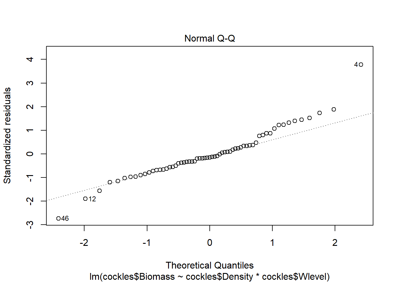
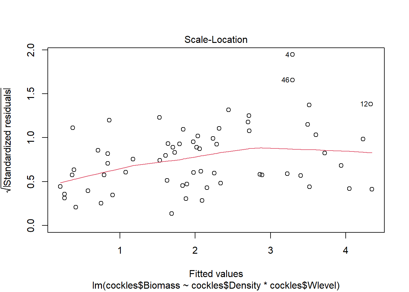
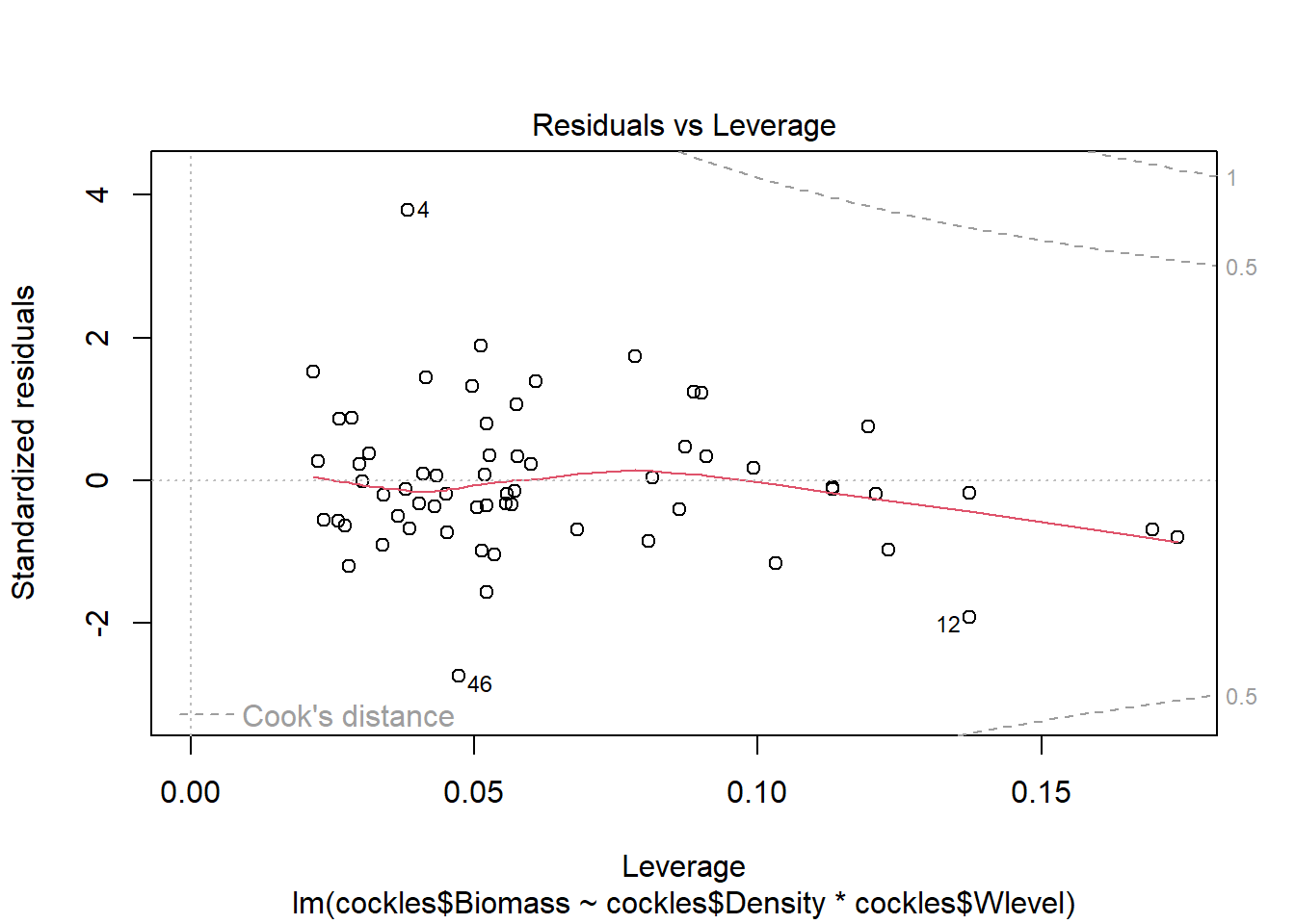
plot(cockles.bdw)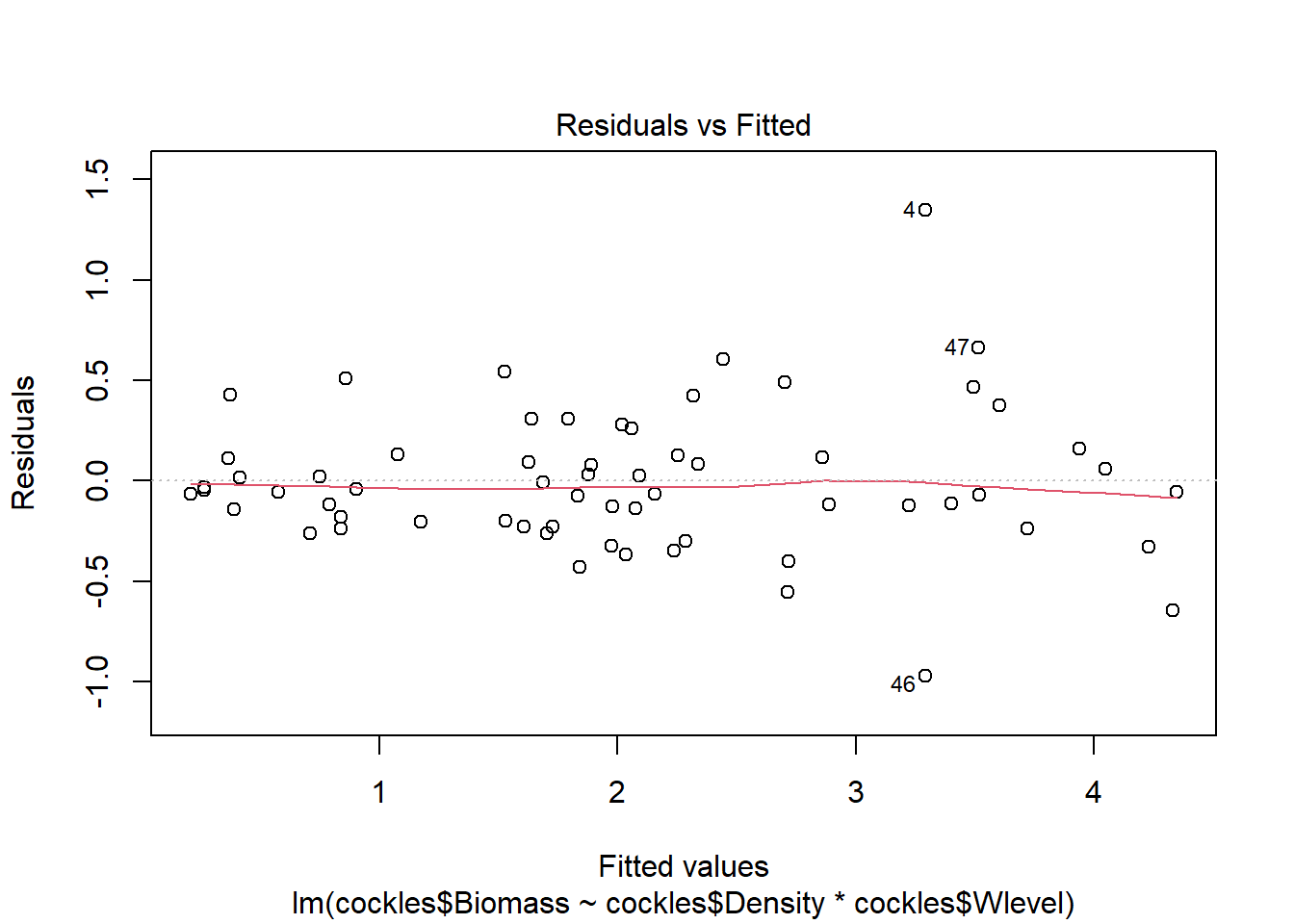
Excluding outliers (4, 46) the residuals show fairly constant variance, and there are no points with residual values greater than \(\pm 2\). There is no indication of non-linearity in the relationship.
The normal qq plot looks ok, the standardised residuals are fairly close to the standard normal quantiles. There is some separation at the more extreme quantiles but this is typically expected.
There are a few outliers with square root standardised residuals around 1.5 to 2 (corresponding to 2.25 to 4 when squared).
The fourth plot indicates a couple of highly influential points - observations 4, 12 and 46. The influence of points 4 and 46 is due to large standardised residual values (they are outliers). This may be due to measurement or transcription errors, however their values are not dramatically different from the other observations. It is more likely that there is additional natural variation that has not been accounted for by our model. Observation 12 has quite a large negative residual value, and is also in a position of high leverage within the data set. It is likely the most influential observation.