4 Infrared Thermography

The development of a non-invasive tool (infrared thermography) to measure stress and pain in animals has significant applications in assuring the welfare standards of the New Zealand agricultural industry and boosting the value of its products in overseas markets. Here we are interested in stress involved in the disbudding (removal of horns) of cattle.

This lesson investigates the emotional and or stress responses of cattle during disbudding using four different treatment options. The original research was carried out by Mairi Stewart (AgResearch, Ruakura).

Data

Data Summary

30 observations

6 variables

Variable	Type	Information
Tag	Categorical	Cow ID, used for identification rather than analysis.
Trt num	Categorical	4 levels: 1,2,3,4. Equivalent to Trt.
Trt	Categorical	4 levels: Control, LA, DB, LADB . Treatment type.
Base eye temperature	Continuous	Baseline eye temperature in (°C).
Temperature in first 3 mins post treatment	Continuous	Measured in (°C).
Change in eye temperature	Continuous	Eye temp 3 mins post treatment minus baseline (°C).

There is 1 file associated with this presentation. It contains the data you will need to complete the lesson tasks.

Download Disbud stress.xls

Video

Objectives

Learning Objectives

New skills and concepts:

Experimental design.
Confidence interval for difference in means.
Bootstrap confidence intervals for mean and difference in means.

Reinforcing skills and concepts seen in earlier lessons:

Read and format data.
Introduction to plotting.
Confidence intervals for means.
Linear regression and ANOVA for single predictor.

Tasks

0. Read and Format data

0a. Read in the data

First check you have installed the package readxl (see Section 2.6) and set the working directory (see Section 2.1), using instructions in Getting started with R.

Load the data into R.

Important Information

Name your data disbud for easier reference later.

Previous Lesson

To load the data in R we run code analogous to Task 0 in Cockles Section 3.0.1

This creates a data frame containing data from a study investigating the effects of 4 different disbudding treatments on dairy calves.

The code has been hidden initially, so you can try to load the data yourself first before checking the solutions.

Code

#loads readxl package
library(readxl) 

#loads the data file and names it disbud
disbud<-read_xls("Disbud stress.xls")

#view beginning of data frame
head(disbud)

Code

#loads readxl package
library(readxl)

Warning: package 'readxl' was built under R version 4.2.2

Code

#loads the data file and names it disbud
disbud<-read_xls("Disbud stress.xls")

New names:
• `` -> `...7`
• `` -> `...8`
• `` -> `...9`
• `` -> `...10`
• `` -> `...11`
• `` -> `...12`
• `` -> `...13`

Code

#view beginning of data frame
head(disbud)

# A tibble: 6 × 13
    Tag `Trt num` Trt     Base e…¹ Tempe…² Chang…³ ...7  ...8  ...9  ...10 ...11
  <dbl>     <dbl> <chr>      <dbl>   <dbl>   <dbl> <lgl> <chr> <chr> <chr> <chr>
1  5124         1 Control     37.0    37.2  0.212  NA    Trea… <NA>  <NA>  <NA> 
2  5659         1 Control     37.1    36.8 -0.303  NA    DB    Disb… <NA>  <NA> 
3  5656         1 Control     37.4    37.6  0.238  NA    LADB  Disb… <NA>  <NA> 
4  5677         1 Control     37.9    37.8 -0.0871 NA    Cont… Sali… <NA>  <NA> 
5  5132         1 Control     37.6    37.8  0.261  NA    LA    Loca… <NA>  <NA> 
6  5950         1 Control     38.1    37.9 -0.157  NA    <NA>  <NA>  <NA>  <NA> 
# … with 2 more variables: ...12 <chr>, ...13 <chr>, and abbreviated variable
#   names ¹`Base eye temperature (°C)`,
#   ²`Temperature in first 3 mins post treatment (°C)`,
#   ³`Change in eye temperature (°C)`
# ℹ Use `colnames()` to see all variable names

In this study 30 calves were allocated to one of 4 treatments for disbudding then stress levels were monitored using infrared thermography (a non-invasive method which measured eye-temperature).

The variables recorded are Tag, Trt num (treatment number), Trt(treatment),Base eye temperature (°C), Temperature in first 3 mins post treatment (°C), and Change in eye temperature (°C). The four treatment types recorded are Control, LA (local anaesthetic injection, mock disbudding), DB (disbudded with saline injection) and LADB (disbudded with local anaesthetic injection).

0b. Format the data

Tidy up the data frame by specifying Trt as a factor variable and renaming some of the variables for easier reference later.

Important Information

The Tag and Trt variables can keep the same name, but it will be easier to refer to the other variables later if we remove the spaces and abbreviate their names to TrtNum, BaseEyeTemp, PostTreatEyeTemp and ChangeEyeTemp. Make sure you specify the new names in the same order as the original data frame columns.

Previous Lesson

You can convert code from Task 0 in Cockles Section 3.0.1, so give this a go first.

Code

#reassign as factor variable
disbud$Trt<-as.factor(disbud$Trt)

#rename columns for easier reference
colnames(disbud)<-c("Tag","TrtNum","Trt","BaseEyeTemp","PostTreatEyeTemp","ChangeEyeTemp")

Code

#reassign as factor variable
disbud$Trt<-as.factor(disbud$Trt)

#rename columns for easier reference
colnames(disbud)<-c("Tag","TrtNum","Trt","BaseEyeTemp","PostTreatEyeTemp","ChangeEyeTemp")

Another data tidying step we can take is removing extra columns and NAs.

Code

#overwrite the original disbud data frame with the data frame without NAs using na.omit()
#subsetting with [] to only include the first 6 columns, the remaining 7 have comments/information we do not need
disbud<-na.omit(disbud[,c(1:6)])

Code

#overwrite the original disbud data frame with the data frame without NAs using na.omit()
#subsetting with [] to only include the first 6 columns, the remaining 7 have comments/information we do not need
disbud<-na.omit(disbud[,c(1:6)])

Discuss the importance of a randomised design.

How many treatments are present?

Why might one of the treatments have only 6 cattle?

Is there a control treatment that other treatments are compared with?

See video Section 4.1

A randomised design is important as it controls the effects of potential confounding variables (in the present study this could include factors such as breed of calf, temperament). This allows researchers to detect a true effect/relationship between the variables of interest if one does exist.

There were 4 treatments present in this study - handling only, local anaesthetic only, disbudding only, and disbudding with local anaesthetic.

The disbudding only treatment group had only 6 cattle as this was the minimum number required to detect a true difference between groups (with 30 calves across groups). As disbudding without local anaesthetic was the most painful treatment group, for ethical reasons the number of calves were limited here.

There were 2 control treatments that the others were compared with. These were handling only and local anaesthetic only.

2. Box Plot, Scatter Plot

It is important to know what our data looks like, as it may help us to understand the results of the calculations that we will be doing later on.

Plot ChangeEyeTemp against the four Trt groups.

What can you see from the graphs?

Code

#plot() function returns a box plot for each treatment as this is a categorical variable
plot(disbud$Trt, disbud$ChangeEyeTemp)

Have a look at the help file for the plot() function to figure out how to produce a scatter plot instead.

Code

#plot() function returns a box plot for each treatment as this is a categorical variable
plot(disbud$Trt, disbud$ChangeEyeTemp)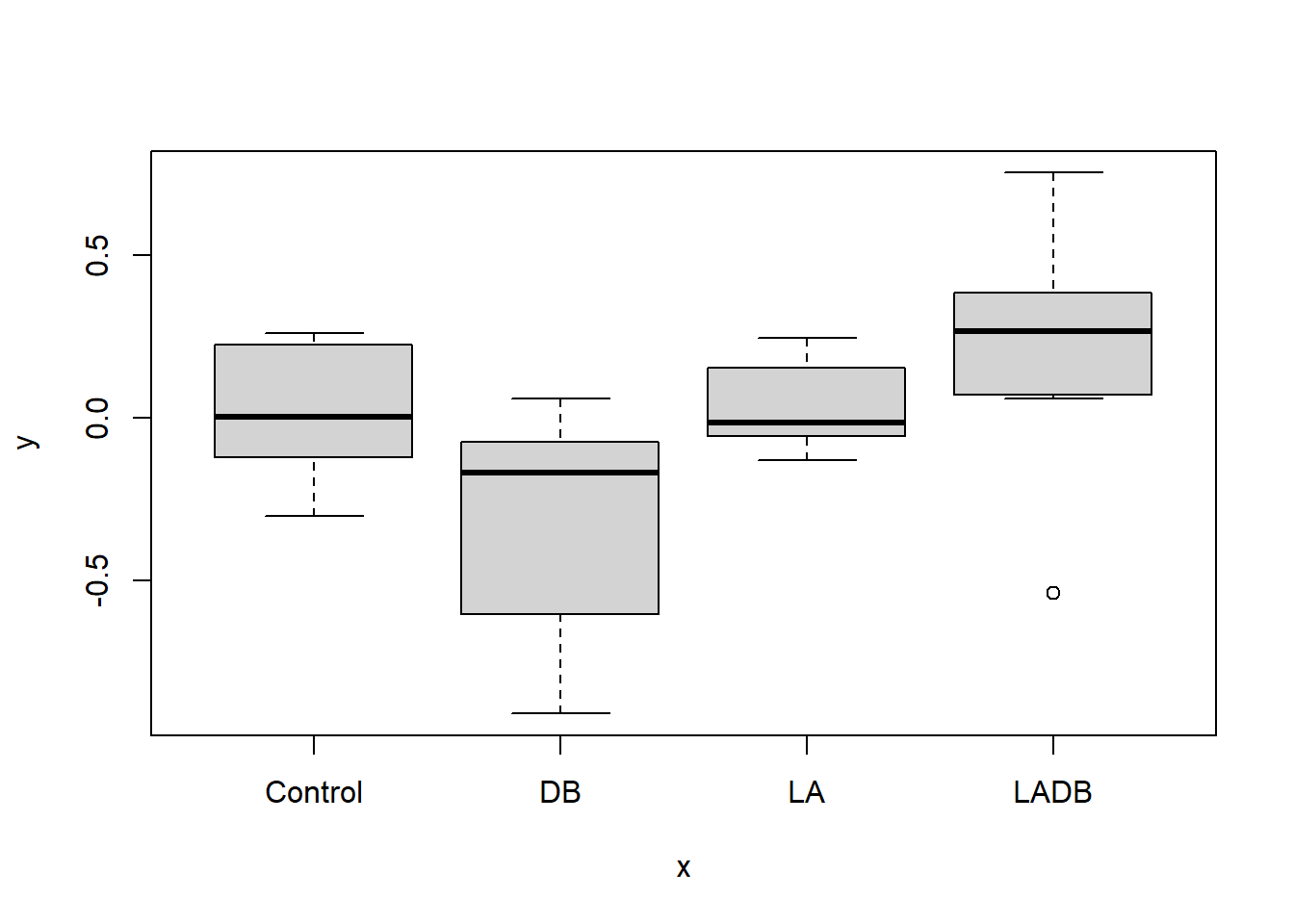

Code

#can see individual points using plot.default() instead
plot.default(disbud$Trt, disbud$ChangeEyeTemp)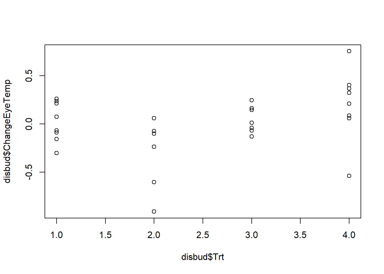

Previous Lesson

See Task 1a. (Section 3.0.2) in Cockles for interpretation of box plots.

3. Confidence Interval (mean)

Calculate the mean ChangeEyeTemp and the standard error for each Trt mean (SEM).

Using these summary statistics and the formula below, calculate a 95% confidence interval for the mean change in eye temperature for each treatment group (use a large sample value of 1.96 or 2).

\[ \overline{x} \pm 1.96 * \frac{\sigma_x}{\sqrt{n}}\]

Previous Lesson

Use the same methods as Task 1c. in Cockles Section 3.0.2.

What do you conclude?

Code

#estimate of the mean change in eye temperature for control cattle
mean(disbud$ChangeEyeTemp[disbud$Trt=="Control"]) 

#estimate of the standard error of the mean change in eye temperature for control cattle
sd(disbud$ChangeEyeTemp[disbud$Trt=="Control"])/sqrt(length(disbud$ChangeEyeTemp[disbud$Trt=="Control"]))

Calculate these components for the LA, DB, and LADB Trt groups.

Code

#eye temperature for control cattle
m<-mean(disbud$ChangeEyeTemp[disbud$Trt=="Control"]) 

se<-sd(disbud$ChangeEyeTemp[disbud$Trt=="Control"])/sqrt(length(disbud$ChangeEyeTemp[disbud$Trt=="Control"]))

m-1.96*se

[1] -0.1220748

Code

m+1.96*se

[1] 0.1647258

Code

#eye temperature for local anaesthetic cattle
m<-mean(disbud$ChangeEyeTemp[disbud$Trt=="LA"]) 
se<-sd(disbud$ChangeEyeTemp[disbud$Trt=="LA"])/sqrt(length(disbud$ChangeEyeTemp[disbud$Trt=="LA"]))

m-1.96*se

[1] -0.05590293

Code

m+1.96*se

[1] 0.1273838

Code

#eye temperature for disbudding cattle
m<-mean(disbud$ChangeEyeTemp[disbud$Trt=="DB"]) 
se<-sd(disbud$ChangeEyeTemp[disbud$Trt=="DB"])/sqrt(length(disbud$ChangeEyeTemp[disbud$Trt=="DB"]))

m-1.96*se

[1] -0.6067618

Code

m+1.96*se

[1] -0.0143709

Code

#eye temperature for disbudding and local anaesthetic cattle
m<-mean(disbud$ChangeEyeTemp[disbud$Trt=="LADB"]) 
se<-sd(disbud$ChangeEyeTemp[disbud$Trt=="LADB"])/sqrt(length(disbud$ChangeEyeTemp[disbud$Trt=="LADB"]))

m-1.96*se

[1] -0.04967224

Code

m+1.96*se

[1] 0.4657519

Previous Lesson

See Task 1c. (Section 3.0.2) in Cockles for interpretation of confidence intervals.

In practice a t-value (calculated using the function qt()) should be used for confidence intervals as we have small samples for each of the treatments. The t-value would have 8-1=7 degrees of freedom (df) for treatments 1, 2, and 4, but only 6-1 df for treatment 3.

The function t.test() carries out this entire process automatically. You can try this for an extension.

Previous Lesson

See Cockles Task 1d. Section 3.0.2 (your answers will be slightly different to those calculated by hand, as explained here).

4. Bootstrap Confidence Interval, Histogram (mean)

For each Trt, we want to calculate the bootstrap confidence interval for the mean ChangeEyeTemp.

The bootstrap technique involves randomly sampling a new dataset from the original sampled data. This creates a large number of datasets, that may have been seen if the experiment had been repeated many times (i.e. creates new datasets based on the original dataset).

This can be done in R using the boot package.

Previous Lesson

Install new packages using instructions in Getting started with R Section 2.6.

What distribution do the means of the bootstrap samples appear to follow?

How do the bootstrap estimates of the mean for each treatment group compare to the treatment means we calculated previously? Do the bootstrap confidence intervals lead to the same conclusions as before (for each treatment group)?

Code

library(boot)

#set seed so you get the same results when running again
set.seed(4)  

#function that calculates the mean from the bootstrapped samples
meanFun<-function(data,indices){  
  dataInd<-data[indices,]  #sample rows with replacement from the data
  meandata<-mean(dataInd$ChangeEyeTemp) #calculate statistic of interest, in this case the mean, from the sample
  return(meandata)
}

#use the boot() function to bootstrap mean change in eye temp for control cattle
#create object called meanBoot with the output of the bootstrapping procedure
meanBoot<-boot(disbud[disbud$Trt=="Control",],statistic=meanFun, R=10000)

After running the bootstrap sampling, we can view summary statistics of the results by calling the object.

Code

meanBoot

From the \(\verb!Bootstrap Statistics!\) output we can calculate a normal 95% confidence interval using the estimate of \(\verb!t1*!\) and the \(\verb!std. error!\).

Important Information

You will have slightly difference results for the standard error due to the nature of bootstrapping, so should modify the numbers below to match your output.

Code

lower<-0.02132551-1.96*0.06804017
upper<-0.02132551+1.96*0.06804017

It is also useful to produce a graph of the distribution of the results.

This graph shows the distribution of the mean of the bootstrap samples with a density curve and 95% confidence interval limits plotted on top.

Code

#plot density (freq=F) histogram of bootstrap results
hist(meanBoot$t,freq=F) 

#add a smoothed line to show the distribution
lines(density(meanBoot$t))

#add vertical lines with lower and upper confidence limits
abline(v=c(lower,upper))

Code

library(boot)

Warning: package 'boot' was built under R version 4.2.2

Code

#set seed so you get the same results when running again
set.seed(4)  

#function that calculates the mean from the bootstrapped samples
meanFun<-function(data,indices){  
  dataInd<-data[indices,]  #sample rows with replacement from the data
  meandata<-mean(dataInd$ChangeEyeTemp) #calculate statistic of interest, in this case the mean, from the sample
  return(meandata)
}

#use the boot() function to bootstrap mean change in eye temp for control cattle
#create object called meanBoot with the output of the bootstrapping procedure
meanBoot<-boot(disbud[disbud$Trt=="Control",],statistic=meanFun, R=10000)

After running the bootstrap sampling, we can view summary statistics of the results by calling the object.

Code

meanBoot


ORDINARY NONPARAMETRIC BOOTSTRAP


Call:
boot(data = disbud[disbud$Trt == "Control", ], statistic = meanFun, 
    R = 10000)


Bootstrap Statistics :
      original        bias    std. error
t1* 0.02132551 -8.071731e-05  0.06858631

From the \(\verb!Bootstrap Statistics!\) output we can calculate a normal 95% confidence interval using the estimate of \(\verb!t1*!\) and the \(\verb!std. error!\).

Important Information

You will have slightly difference results for the standard error due to the nature of bootstrapping, so should modify the numbers below to match your output.

Code

lower<-0.02132551-1.96*0.06804017
upper<-0.02132551+1.96*0.06804017
lower

[1] -0.1120332

Code

upper

[1] 0.1546842

It is also useful to produce a graph of the distribution of the results.

This graph shows the distribution of the mean of the bootstrap samples with a density curve and 95% confidence interval limits plotted on top.

Code

#plot density (freq=F) histogram of bootstrap results
hist(meanBoot$t,freq=F) 

#add a smoothed line to show the distribution
lines(density(meanBoot$t))

#add vertical lines with lower and upper confidence limits
abline(v=c(lower,upper))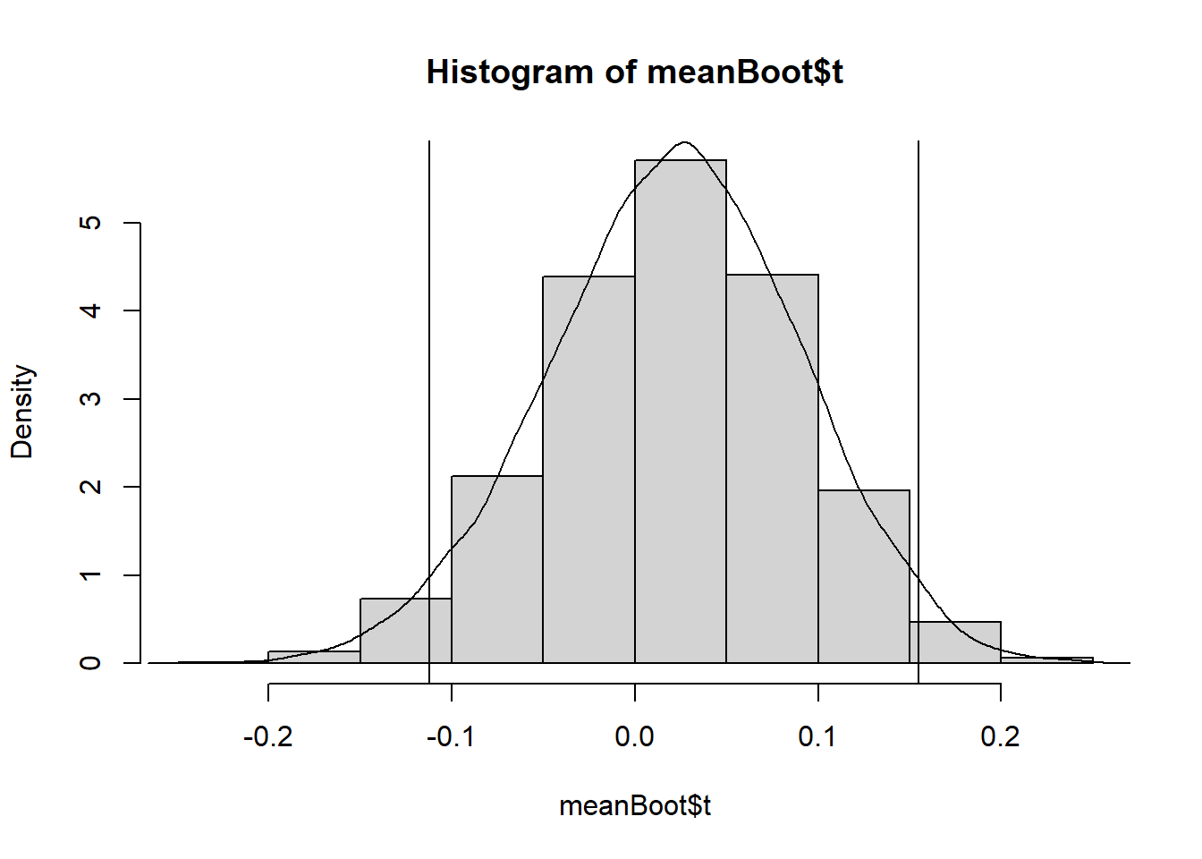

The means of bootstrapped samples follow a normal distribution, symmetric around a mean of 0.02132551. This mean of means matches the mean of the control treatment group we calculated earlier, and the distribution of bootstrapped mean estimates around it give an indication of the amount of variability in our estimate due to sampling.

The bootstrap confidence interval is similar to the one calculated earlier and includes both positive and negative values so leads to the same conclusion. There is no evidence to conclude a significant change in mean eye temperature for control cattle.

Repeat the bootstrapping above for the other Trt groups, and produce histograms of their results.

5. Confidence Interval (difference in means)

To compare the Trt means for the DB and LABD treatments we want to set up a 95% confidence interval for the difference between the means using an unpaired t.test().

Previous Lesson

You can modify code from Task 3b. of Cockles Section 3.0.4.

What conclusion can be drawn from our confidence intervals in regard to the effect of the local anaesthetic?

Code

#first test if variances are equal
var.test(disbud$ChangeEyeTemp[disbud$Trt=="DB"], disbud$ChangeEyeTemp[disbud$Trt=="LADB"], 
         alternative = "two.sided") 

#no significant evidence against null hypothesis that variances are equal, use var.equal=T in t test

#compare the change in eye temperature for disbudding with saline and disbudding with local anaesthetic. 
#paired=FALSE indicates independent samples.
t.test(disbud$ChangeEyeTemp[disbud$Trt=="DB"],disbud$ChangeEyeTemp[disbud$Trt=="LADB"],
    paired=FALSE,var.equal=T)

Calculate the difference in means using the \(\verb!sample estimates:!\) section of the output above.

Code

#first test if variances are equal
var.test(disbud$ChangeEyeTemp[disbud$Trt=="DB"], disbud$ChangeEyeTemp[disbud$Trt=="LADB"], 
         alternative = "two.sided")


    F test to compare two variances

data:  disbud$ChangeEyeTemp[disbud$Trt == "DB"] and disbud$ChangeEyeTemp[disbud$Trt == "LADB"]
F = 0.99071, num df = 5, denom df = 7, p-value = 0.9712
alternative hypothesis: true ratio of variances is not equal to 1
95 percent confidence interval:
 0.1874494 6.7894420
sample estimates:
ratio of variances 
         0.9907146

Code

#no significant evidence against null hypothesis that variances are equal, use var.equal=T in t test

#compare the change in eye temperature for disbudding with saline and disbudding with local anaesthetic. 
#paired=FALSE indicates independent samples.
t.test(disbud$ChangeEyeTemp[disbud$Trt=="DB"],disbud$ChangeEyeTemp[disbud$Trt=="LADB"],
    paired=FALSE,var.equal=T)


    Two Sample t-test

data:  disbud$ChangeEyeTemp[disbud$Trt == "DB"] and disbud$ChangeEyeTemp[disbud$Trt == "LADB"]
t = -2.5871, df = 12, p-value = 0.02378
alternative hypothesis: true difference in means is not equal to 0
95 percent confidence interval:
 -0.95536854 -0.08184378
sample estimates:
 mean of x  mean of y 
-0.3105663  0.2080398

Code

#difference in means
-0.3105663-0.2080398

[1] -0.5186061

Previous Lesson

See Task 3c. (Section 3.0.4) in Cockles for interpreting confidence intervals of the difference between means.

Construct confidence intervals for the other four differences in means using t.test().

6. Bootstrap Confidence Interval, Histogram (difference in means)

Calculate the bootstrap confidence interval for the difference between the two Trt means in Task 5.

Previous Task

This uses the procedure from Task 4, with a few adjustments.

How does the bootstrap estimate of the mean difference between DB and LADB compare with the estimate of the mean difference found in Task 5? Does the bootstrap confidence interval lead to the same conclusion as before?

Was this outcome expected?

Code

library(boot)

#set seed so you get the same results when running again
set.seed(16) 

#function that calculates the difference in means from the bootstrapped samples
meandiffFun<-function(data,indices){  
  data1<-data[data$Trt=="DB",] #subset data by treatment levels, then sample from these
  dataInd1<-data1[indices,]
  data2<-data[data$Trt=="LADB",] #subset data by treatment levels, then sample from these
  dataInd2<-data2[indices,]
  meandiff<-mean(dataInd1$ChangeEyeTemp,na.rm=T)-mean(dataInd2$ChangeEyeTemp,na.rm=T) #calculate difference in means for the samples. Use na.rm=T to remove NAs
  return(meandiff)
}

#bootstrap difference in mean change in eye temp for DB and LADB cattle.
#create object called meandiffBoot with the output of the bootstrapping procedure
meandiffBoot<-boot(disbud[disbud$Trt=="DB"|disbud$Trt=="LADB",],statistic=meandiffFun, R=10000)

Code

#plot density histogram of bootstrap results
hist(meandiffBoot$t,freq=F) 

#add a smoothed line to show the distribution
lines(density(meandiffBoot$t,na.rm=T))

View the summary output and calculate the confidence interval, then add this to your plot above using the abline() function).

Previous Task

See Task 4.

Notice that the bootstrap mean and confidence interval are both negative. What causes the negative difference between the means and could we make it a positive difference?

Code

library(boot)

#set seed so you get the same results when running again
set.seed(16) 

#function that calculates the difference in means from the bootstrapped samples
meandiffFun<-function(data,indices){  
  data1<-data[data$Trt=="DB",] #subset data by treatment levels, then sample from these
  dataInd1<-data1[indices,]
  data2<-data[data$Trt=="LADB",] #subset data by treatment levels, then sample from these
  dataInd2<-data2[indices,]
  meandiff<-mean(dataInd1$ChangeEyeTemp,na.rm=T)-mean(dataInd2$ChangeEyeTemp,na.rm=T) #calculate difference in means for the samples. Use na.rm=T to remove NAs
  return(meandiff)
}

#bootstrap difference in mean change in eye temp for DB and LADB cattle.
#create object called meandiffBoot with the output of the bootstrapping procedure
meandiffBoot<-boot(disbud[disbud$Trt=="DB"|disbud$Trt=="LADB",],statistic=meandiffFun, R=10000)

Code

#plot density histogram of bootstrap results
hist(meandiffBoot$t,freq=F) 

#add a smoothed line to show the distribution
lines(density(meandiffBoot$t,na.rm=T))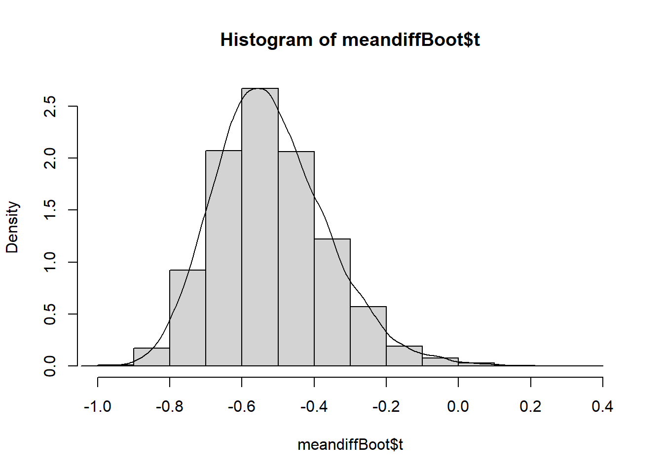

View the summary output and calculate the confidence interval, then add this to your plot above using the abline() function).

Code

meandiffBoot


ORDINARY NONPARAMETRIC BOOTSTRAP


Call:
boot(data = disbud[disbud$Trt == "DB" | disbud$Trt == "LADB", 
    ], statistic = meandiffFun, R = 10000)


Bootstrap Statistics :
      original        bias    std. error
t1* -0.5186062 -0.0004171598   0.1558538

Important Information

You will have slightly difference results for the standard error due to the nature of bootstrapping, so should modify the numbers below to match your output.

Code

lower<--0.5186062-1.96*0.1558538
upper<--0.5186062+1.96*0.1558538
lower

[1] -0.8240796

Code

upper

[1] -0.2131328

Code

#plot density (freq=F) histogram of bootstrap results
hist(meandiffBoot$t,freq=F) 

#add a smoothed line to show the distribution, remove NAs
lines(density(meandiffBoot$t,na.rm=TRUE))

#add vertical lines with lower and upper confidence limits
abline(v=c(lower,upper))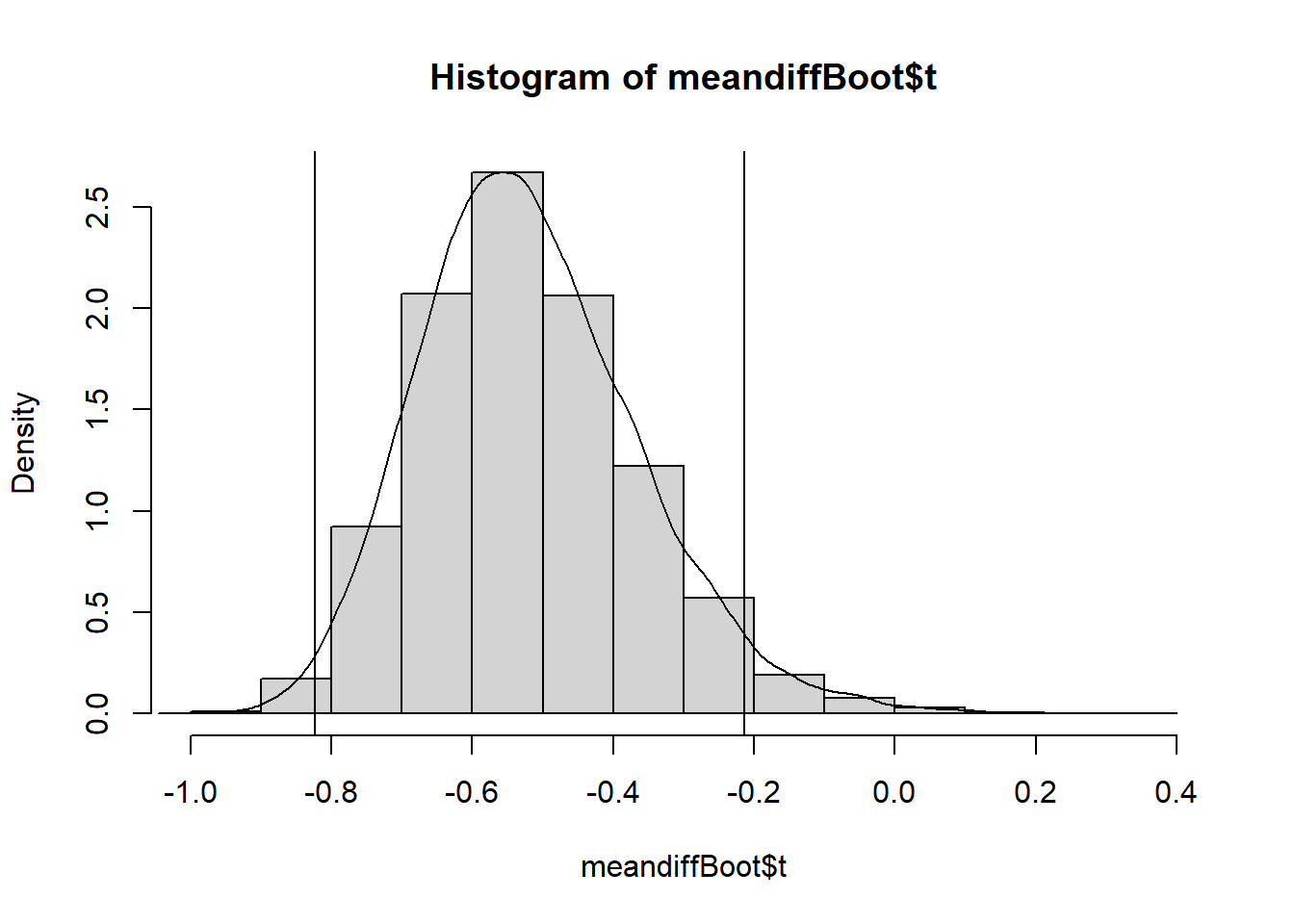

The bootstrapped difference in means follows a near normal distribution around a mean of -0.5186062 with right skew (right side tail). This mean of means matches the difference in means of the disbudding and local anaesthetic with disbudding treatment groups we calculated earlier, and the distribution of bootstrapped difference in mean estimates around it give an indication of the amount of variability in our estimate due to sampling.

The bootstrap confidence interval is narrower than the one calculated earlier and includes only negative values so leads to the same conclusion. There is significant evidence to conclude a difference in mean eye temperature between disbudding and disbudding with local anaesthetic.

As the earlier confidence interval nearly included 0 (upper limit of -0.0818) and bootstrap confidence intervals always differ slightly from those calculated by hand or t.test() this outcome was not necessarily certain.

Construct bootstrap confidence intervals and histograms of the results for the other four differences in means.

7. Simple Linear Regression, ANOVA

An alternative to pairwise bootstrapping for the comparison of means is the Analysis of Variance procedure: ANOVA. This tests for a significant difference between 2 or more groups, and can test for a significant difference between all 4 Trt groups at once.

Fit a linear model for the effect of Trt on ChangeEyeTemp and then carry out ANOVA for this object.

Previous Lesson

Cockles Task 3a. Section 3.0.4.

Report your findings. What conclusions can you draw from the results you have obtained so far?

Code

#fitted linear model
disbud.trt<-lm(disbud$ChangeEyeTemp~disbud$Trt)
summary(disbud.trt)

#calculate ANOVA object
anova(disbud.trt) 

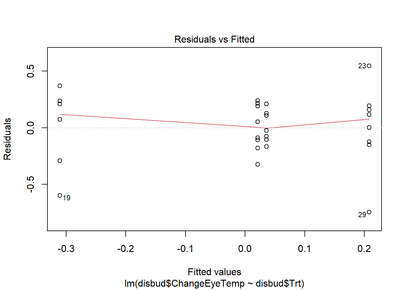
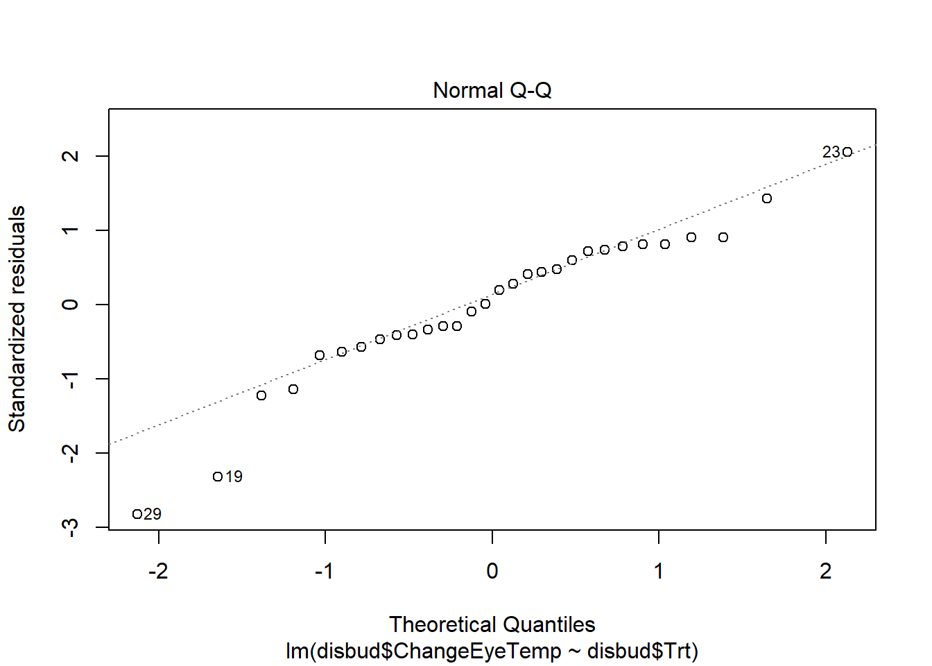
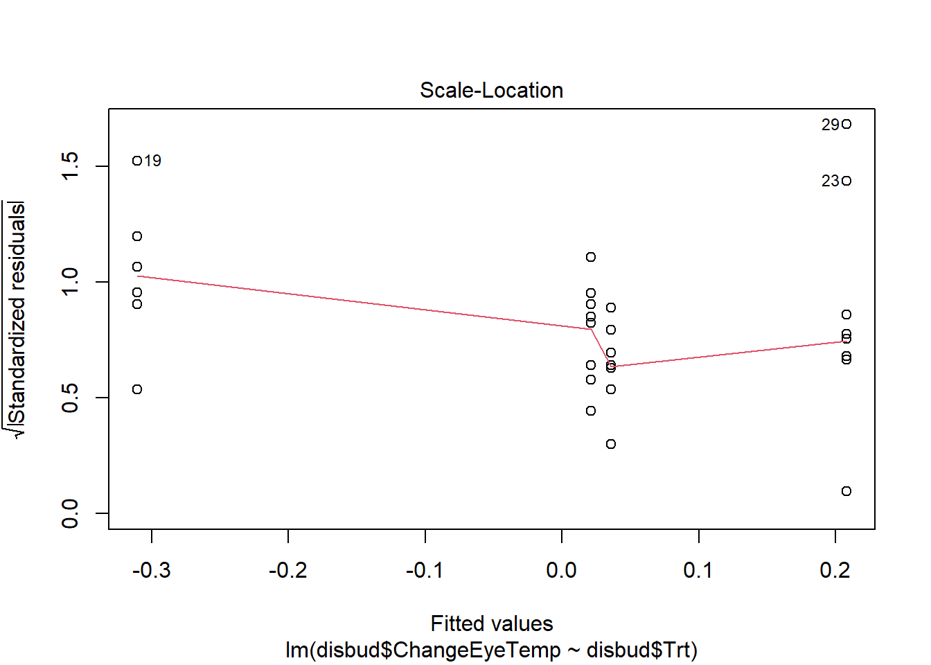
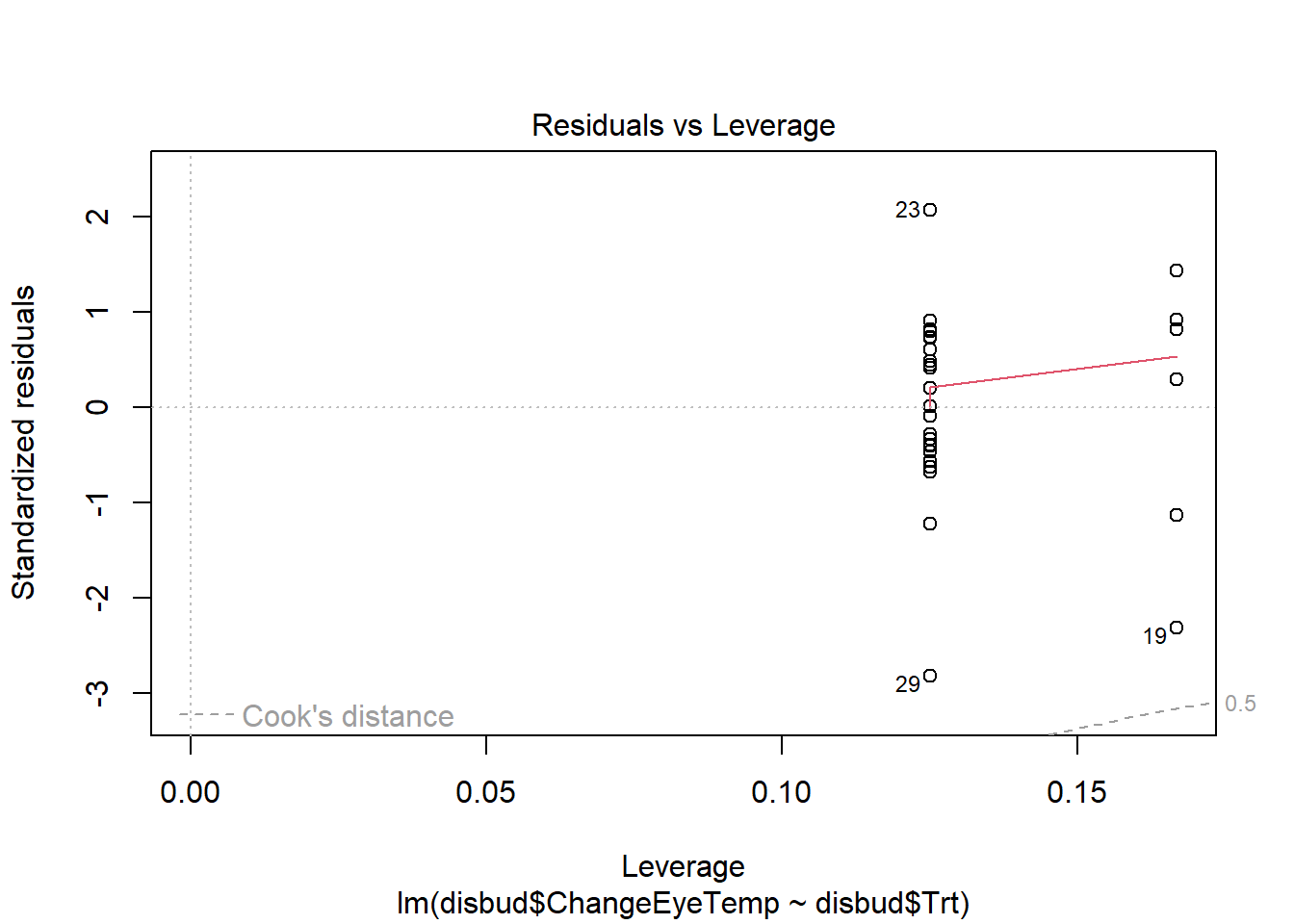
#residual checks
plot(disbud.trt)

Code

#fitted linear model
disbud.trt<-lm(disbud$ChangeEyeTemp~disbud$Trt)
summary(disbud.trt)


Call:
lm(formula = disbud$ChangeEyeTemp ~ disbud$Trt)

Residuals:
     Min       1Q   Median       3Q      Max 
-0.74582 -0.11896  0.02706  0.19426  0.54555 

Coefficients:
               Estimate Std. Error t value Pr(>|t|)  
(Intercept)     0.02133    0.09989   0.213   0.8326  
disbud$TrtDB   -0.33189    0.15259  -2.175   0.0389 *
disbud$TrtLA    0.01441    0.14127   0.102   0.9195  
disbud$TrtLADB  0.18671    0.14127   1.322   0.1978  
---
Signif. codes:  0 '***' 0.001 '**' 0.01 '*' 0.05 '.' 0.1 ' ' 1

Residual standard error: 0.2825 on 26 degrees of freedom
Multiple R-squared:  0.3109,    Adjusted R-squared:  0.2314 
F-statistic: 3.911 on 3 and 26 DF,  p-value: 0.01979

Code

#calculate ANOVA object
anova(disbud.trt)

Analysis of Variance Table

Response: disbud$ChangeEyeTemp
           Df Sum Sq  Mean Sq F value  Pr(>F)  
disbud$Trt  3 0.9366 0.312200   3.911 0.01979 *
Residuals  26 2.0755 0.079826                  
---
Signif. codes:  0 '***' 0.001 '**' 0.01 '*' 0.05 '.' 0.1 ' ' 1

Code

#residual checks
plot(disbud.trt)

Previous Lesson

See Tasks 3a. (Section 3.0.4) and 5b. (Section 3.0.6) in Cockles for analysis of simple linear regression and residual checking.